|
As mentioned above, if you enter a value in a cell and press
Enter, you move focus to the cell under it or if you press Tab, you move focus
to the cell on the right side. As an alternative, you can indicate the sequence
of cells you want to follow so that, when you press Enter or Tab, the focus
would not necessarily move to the right or the cell under but rather to the cell
in the sequence of your choice. To do this:
- Randomly select the sequence of cells you want. In other words, click the
first cell in your intended sequence, press and hold Ctrl, then click each
cell in the desired order
- While still holding Ctrl, once again click the cell that will be the
first, and release Ctrl
- Type the desired value in that first cell
- Press Enter or Tab
- Type the value in the next cell of the sequence
- Repeat steps d and e
- When you have finished, either press one of the arrow keys or click a cell
that is not in the sequence
|
 |
In Microsoft Excel, you can enter a common value for the
same cell address in different worksheets. To do this, first select the
worksheets as we saw in Lesson 5. Click the intended cell and type the desired
value
If you type something, it goes into the
active cell.
If you click a cell and start typing, the new entry will replace the content of that cell, whether that cell had data or not, this could be advantageous or disastrous.
To prevent a cell from being edited by the user, you can protect it and lock its content.
Data you type in a cell can consist of any kinds of characters, letters, numbers, etc. Sometimes, a long text will look like covering more than one cell; unless you merge cells, the text you type goes into one cell regardless of the length of the text.
A cell can contain as many as 32767 characters.
Data that you type in a worksheet is in fact entered in cells, except when you are drawing.
Unlike a traditional word processor, Microsoft Excel has a unique way of treating text and considering any data you type in a cell.
Data entered in a cell is confined to that cell. If you type text that is longer than the cell's width, the content will display fine, giving the impression that the text is covering more than one cell or that the cell on the right side is no more available. Data you type is always in its cell. If you type anything in a cell, its content will take priority in displaying its
content. Therefore the content of the left cell will appear cut. That's why you should be very familiar with the way a cell (any cell) displays its
data, and how every cell relates to the others.
|
 Practical Learning:
Entering Text Into Cells Practical Learning:
Entering Text Into Cells
|
|
- Start Microsoft Excel with its default workbook
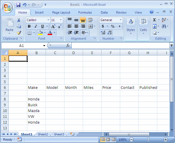
- Click Cell B8 and type Honda
- Press Enter
- Type Buick and press Enter
- Type Mazda and press the down arrow key
- Type Folks Wagon
- On the Quick Access toolbar, click the Undo button
 . That deletes the content of cell
B11 . That deletes the content of cell
B11
- Type VW and press the down arrow key
- Type h and notice that the cell is auto-completed with Honda
- Click Cell B6, type Make and press the right arrow key
- Type Model and press Tab
- Type Month
- Click Cell G6 and type Contact and press Shift + Tab to move focus
to the left cell
- Type rice and click the Enter button

- Type Price and press the left arrow key
- Type Miles and press the right arrow key three times
- Type Published and press Ctrl + Home
- Click Cell C8, type Corolla
- On the Formula Bar, click the Cancel button
 and type Accord
- Click Cell G8, type Brenda and press Enter
- In Cell G9, type David and press the down arrow key
- Type b and press Enter. Notice that Microsoft Excel completed the cell with the word
Brenda
- In cell G11, type Alex and press Enter
- To undo your last action, press Ctrl + Z. Now cell G7 is empty
- Type Juliette and press Enter
- Make sure the Sheet1 tab is selected.
Press and hold Ctrl
- Click Sheet2 and release Ctrl
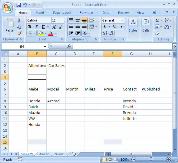
- Click Cell B2
- To enter the same text for the equivalent cells of two worksheets, type Allentown
Car Sales and click Enter
- Click Sheet3 then click Sheet2.
Notice the text in Cell B2
- Click Sheet1
- To determine the only cells intended for the next data entry, click Cell
B4
- Press and hold Ctrl
- Click Cells B15, F15, and then B4 again
- Release Ctrl
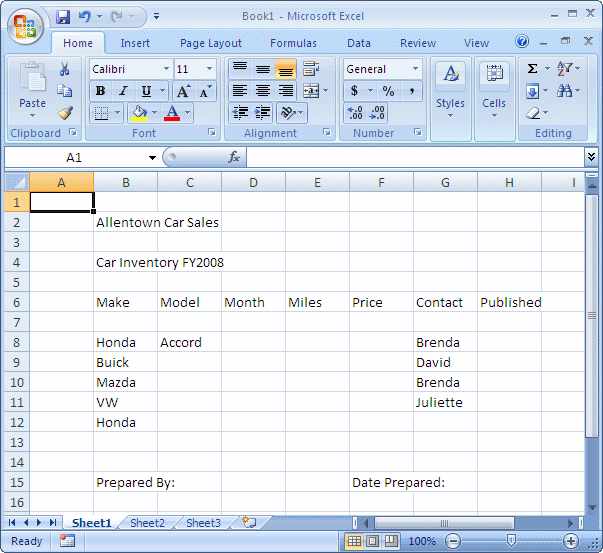
- Type Car Inventory FY2008 and press Enter (twice)
- In Cell B15, type Prepared By: and press Tab
- Type Date Prepared: and press Ctrl + Home
Editing cells content consists of deleting, replacing, altering, or adding something in them. You already know that if you click a cell and start typing, its content
would be replaced with the new entry. If you want to add or subtract something to a cell's
content:
- You can double-click it. This would put the cell in
edit mode and you can then proceed
- Click a cell to give it focus and then press F2. This puts the cell in Edit mode; this time, the
caret is at the end of the text in the cell; then you can proceed
- Click a cell, in the Formula bar, edit the text as you see fit
Whatever technique you use, when you have finished editing a cell, make sure you
move its focus by pressing Tab, Enter, or clicking somewhere else. When you are in
edit mode, the arrow keys are not working, and many actions are not available.
|
 Practical Learning:
Editing Cells Content Practical Learning:
Editing Cells Content
|
|
- Click Cell D6 and type Year to replace the previous cell content
- Click Cell B12 and type Ford to replace the previous entry
- Double-click cell E6. Notice that the caret is positioned in the cell
- Press End, press Backspace to delete s, type age
Now the cell displays Mileage
- Click Cell H6
- Click in the Formula Bar and press Home
- Type Date and press the Space bar to get Date Published
- Press Enter and press Ctrl + Home

- To close the workbook without closing Microsoft Excel, press Ctrl + F4
- When asked whether you want to save, click No
If you have done word processing before, you are probably familiar with techniques of
copying and pasting text from one part of a document to another, or from one document to another.
The same technical approaches are also available in Microsoft Excel.
You can copy the content of one or more cells and store the
value(s) in the clipboard.
In Microsoft Excel 97, you could store only one item at a time in the
clipboard. If you cut or copied something, it would replace the content of
the clipboard with the new selection. In Microsoft Excel 2000, the
clipboard could contain up to twelve items. When the Clipboard toolbar was
functional, you could select copied or cut items from its list of buttons.
If you used more than 12 stored items, the toolbar functioned on a
first-in first-out basis.
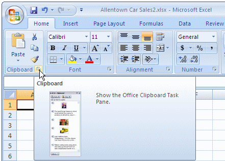
In Microsoft Office 2007, the clipboard is represented
as a window. To display it, on the Ribbon, in the Home tab, and in the
Clipboard section, you can click the more options button:
The Clipboard window can be moved to any location of
your choice on the screen. You can also hide/close it if you don't need
its services. To close it, you can click its Close button or you can click
the more options button.
|
Copying and Pasting Cells
|
|
In Lesson 2, we saw that you could copy one or more columns
and put them to the clipboard. In reality, you would have copied the contents of
the cells under the column header and paste the values of those cells to (an)other
column(s). As a reminder, to copy the contents of the cells of a column to the clipboard:
- Right-click a column header and click Copy
- Click the column header. On the Ribbon, click Home. In the Clipboard
section, click Copy
After copying a column, the values of all of its cells
are available from the clipboard. To paste those cells to another column:
- Right-click the target column header and click Paste
- Click the column header. On the Ribbon, click Home. In the Clipboard
section, click Paste
In Lesson 3, we saw how to copy a row and paste it
somewhere. When you copy a row, you in fact copy the values of the cells
on the right side of its row header. You can then paste the copied values
to another row.
Instead of copying all the cells
of a column or all of the cells of a row, you can copy only one or more
cells to the clipboard:
- To copy the content of a cell:
- Right-click that cell and click Copy. To paste, click the target cell
and simply press Enter, or right-click the target cell and click Paste
- Click the cell. On the Ribbon, click Home. In the Clipboard
section, click Copy. Click the target cell. To paste the content of the
selected cell, click Paste
- Click the cell. Press and hold Ctrl. Position the mouse on one of its
borders. The mouse cursor would be pointing to the top-left and
accompanied by a + sign:

While holding Ctrl, drag to the target cell. When the target cell is
surrounded, release the mouse and release Ctrl
- To copy the contents of various cells, select the cells in a range:
- Right-click the selection and click Copy. Click the top-left cell of the
target cell. To paste, simply press Enter, or right-click a targeted cell
and click Paste
- On the Ribbon, click Home. In the Clipboard
section, click Copy. Click the top-left cell or the target. To paste, in the
Clipboard section of the Ribbon, click Paste
- Press and hold Ctrl. Position the mouse on one of the borders of the
selection. The mouse cursor would be pointing to the top-left and
accompanied by a + sign. While holding Ctrl, drag the group in the
desired direction. When the target cells are surrounded, release the
mouse and release Ctrl
|
 Practical Learning:
Copying Cells Contents Practical Learning:
Copying Cells Contents
|
|
- Open the Grier Summer Camp3 workbook and click the Employment
Application1 if necessary to activate it
- Right-click Cell B8 and click Copy
- Click Cell F8 and press Enter. That pastes First Name to cell F8
- On the Ribbon, click Home if necessary.
In the Clipboard section, click the Clipboard button 
- Right-click Cell B13 and click Copy
- Click Cell F13
- On the Clipboard window, click Home Phone
- Click Cell F15 and type 2)
- Select Cells from C32:G35
In the Clipboard section of the Ribbon, click the Copy button  . That action copies the selected range
to the Clipboard . That action copies the selected range
to the Clipboard
- Click Cell C38
- In the Clipboard window, click the top button to paste the copied
selection
- Cells C38:G41 should still be selected. If the group of Cells
C38:G41 is not selected, select it. Position your mouse on one of the borders of the selected
group until the mouse pointer turns into a
cross
- Press and hold Ctrl
- With the mouse pointer pointing to North West and the mouse now having a small + sign, click and hold the mouse down, then drag towards the lower side of the screen. A small box guides you to know where the selection is
leading
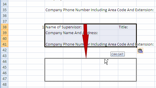
- When you get to C44:G47, release the mouse, then release
Ctrl
- To save the workbook, on the Quick Access toolbar, click the Save button

|
Cutting or Moving the Contents of Cells
|
|
In Lesson 2, we saw how to move a column or a group of
columns from one location to another. In Lesson 3, we saw how to move a row from
one section of the worksheet up or down. Sometimes, instead of moving the whole column or the whole row, you may want to
move only one particular cell or a group of cells. To move the content of a cell to the clipboard
and paste it somewhere:
- Right-click the cell and click Cut. To paste the value of the cell
somewhere, click the target cell and press Enter, or right-click the target
cell and click Paste
- Click the cell. On the Ribbon, click Home. In the Clipboard
section, click Cut. Click the target cell. To paste the cell, in the
Clipboard section of the Ribbon, click Paste
When you move a column or a row, it gets
removed from the previous location and carries its cells to the new location. An
alternative is to
move only a particular group of cells. To move the contents of a group of cells to the clipboard,
select the cells:
- Right-click the group and click Cut. To paste the values of the cells
somewhere, click a target cell and press Enter, or right-click a target cell
and click Paste
- On the Ribbon, click Home. In the Clipboard
section, click Cut. Click the target cell. To paste the cell, in the
Clipboard section of the Ribbon, click Paste
|
 Practical Learning:
Cutting Cells Contents Practical Learning:
Cutting Cells Contents
|
|
- Right-click Cell F18 and click Cut. One more item gets copied to the
Clipboard
- Click Cell D12
On the Clipboard window, click E-Mail
To move a cell, you ask Microsoft Excel to remove its
content from that location to a new location of your choice. When you do this,
only the content of the cell moves, leaving the previous location empty.
To move a cell, first click it to give it focus. Position
the mouse on one of its borders the mouse cursor changes into a cross:

Click and hold your mouse down. Drag up, down, left or right
to the target cell of your choice. A rectangular box that is the same size as
the cell would guide you and assume the position of the mouse where the mouse is
currently over:
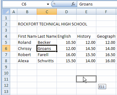
When the cell is positioned where you want, release the
mouse. If you land on a cell that contains something already and that cell is
allowed to receive a value (some cells can be "locked" so they cannot
receive a value), you would receive a warning message box asking you to confirm
that you really want to replace the value in the target cell:
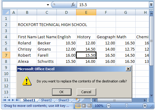
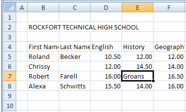
If you click OK, the content of the target value would be
replaced with that of the cell that was moved:
To move more than once cell, first select the cells in a
range (they most be selected as a range). Position the mouse on the border of
the selection until the mouse cursor turns into a cross. Click the drag in the
direction of your choice. A guiding box that is the same size as the group would
guide you. When you get to the new location, release the mouse.
|
 Practical Learning:
Moving a Cell Practical Learning:
Moving a Cell
|
|
- Click Cell D12 to give it focus
- Position the mouse on one of its border until the mouse appears as a
cross. Click and drag to Cell F12
|
Data Entry and Text Management |
|
|
The GoTo, Find, and Replace Dialog Boxes
|
|
When performing data entry or just using a worksheet,
it is pretty easy to identify a cell in the upper section of the document.
Sometimes a cell may be difficult to find. Fortunately, Microsoft Excel
provides the tools to help you locate a cell.
To locate a particular cell in Microsoft Excel, you can use the
Go To dialog box. This dialog box recognizes cells names by applying the same
conventions used by Microsoft Excel. You can get the Go To dialog box from the
main menu under Edit.
The shortcuts to access the Go To dialog box are Ctrl + G or F5.
The Find dialog box allows you to find a word in your worksheet,
either to simply locate a particular word or multiple instances of a word, or to
manipulate a word or groups of words at will.
The Replace dialog box allows you to find a word or group of
words and to replace it with a new word or group of words. Both dialog boxes are
available from the main menu under Edit.
The shortcut for the Find dialog box is Ctrl + F.
The shortcut for the Replace dialog box is Ctrl + H.
|
 Practical Learning: Finding and/or Replacing Cells Content Practical Learning: Finding and/or Replacing Cells Content
|
|
- Open the Grier Summer Camp4 workbook and click the Employment
Application4 tab
- To locate a cell, on the Ribbon, click Home if necessary. In the
Editing section, click Find & Select, and click Go To
- Type F13
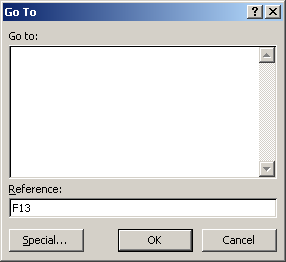
- Click OK
- Press Ctrl + G, that calls the Go To dialog box
- Type C2 and press Enter
- To find a word in the document, in the Editing section of the
Ribbon, click Find & Select, and click Find...
- In the Find What box, type name and click the Find Next
button 8 times. Press Esc to dismiss the Find dialog box
- To find a word and replace it with another word, in the Editing
section of the Ribbon, click Find & Select, and click Replace...
- In the Replace dialog box, in the Find What box, type natural
and press Tab. In the Replace With box, type Nature of
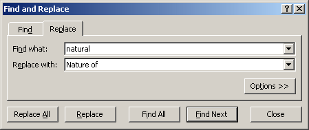
- Click Find Next
- When the first instance of natural is found, click Replace. Click
Replace All
- When all instances have been found and replaced, a message box will
let you know that Microsoft Excel Cannot Find A Match
- Click OK on the message box
- Click Close on the Replace dialog box
- Press Ctrl + S to save the workbook
Although Microsoft Excel is not a word processor, since you
can use it to create text documents such as employment applications, brochures,
time sheets, etc, it can help you correct typing mistakes of various kinds. It
is a good idea to check spelling mistakes in your document before printing it
or sending it for an important business transaction. The check spelling is
done with the help of a Spelling dialog box that will take you step by step
to every word that is questionable. Also, the computer will point out some
suggested words that you can use instead of the one at fault.
You can check your worksheet's spelling during or
after editing, though the latter is better. To check your document:
|
 Practical Learning: Proof Reading the Worksheet Practical Learning: Proof Reading the Worksheet
|
|
- The Grier Summer Camp4 workbook should still be opened.
Access the Employment Application4 worksheet
- On the Ribbon, click Review. In the Proofing section, click Spelling
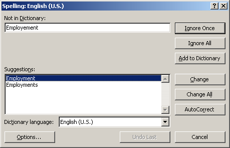
- From the Spelling dialog box, the first suggestion is to change the
word Employement. After making sure that Employment is selected in the
Spelling dialog, then click Change.
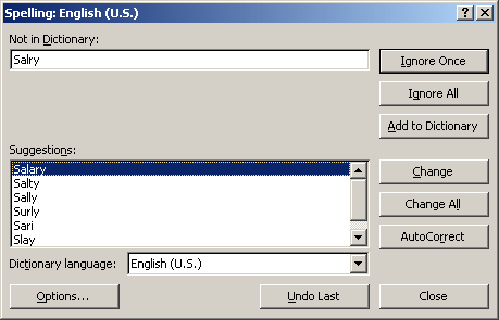
- The next mistake is in the spelling of the word Salary. After making
sure that Salary is selected in the dialog, click Change:
- The next problem is with the word Transportation. From the Spelling
dialog box, in the list of suggested words, click Transportation
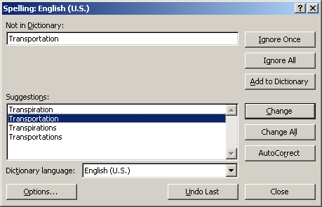
- Click Change
- Accept to Change the word References in cell B27
- In cell B28, accept to change performance
- In cell B30, accept to change the mistake with history
- When the dialog gets to the content of cell B50, select the word
personal instead of personnel to replace personel. Then click Replace
- Also, correct references
- The last problem is with the word sinature. Accept to change it to
Signature

- After the last problem, Microsoft Excel displays a message box
asking whether you want to continue checking at the beginning of the
sheet. Click Yes. Another message box should tell you "The
spelling check is complete for the entire sheet." Click OK
- Press Ctrl + Home to get to the beginning of the worksheet
- Press Ctrl + S to save the workbook
Zooming the work area consists of increasing the ratio of
characters or the contents of the worksheet. Although it does not affect the actual display of the characters sizes or cells contents,
zooming can make the worksheet a little easier to read.
To zoom a worksheet, you have various options:
- Under the horizontal scroll bar is a long bar called Zoom.
This allows you to increase or decrease the
viewed items of the main area of Microsoft Excel
- To change the zoom setting, you can click the Zoom button and
scroll left or right until you get the desired view
Microsoft Excel provides a special dialog box that you can
use to select the zooming magnification. To access it:
- On the the Ribbon, click View. In the Zoom section, click the Zoom
button
- On the Status bar, click the button that shows the
zooming value
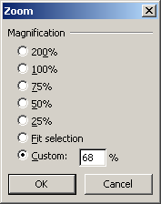
This would open the Zoom dialog box. From there, you
can click one of the radio buttons to select a zooming ratio. To be more
precise, you can click the Custom radio button, then click its text box,
type a number, and click OK.
|
 Practical Learning: Control The Interface’s Zoom Settings
|
|
-
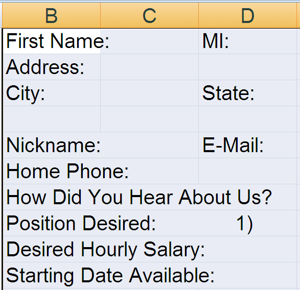
In the worksheet, select cells B8:F21
-
On the Ribbon, click View
-
In the Zoom section, click Zoom to Selection.
Notice that the worksheet displays large characters now
-
In the Zoom section of the Ribbon, click 100%
-
In the lower-right section of the Microsoft Excel, click the spin button and
move it to the right until its value displays 274%

-
Still in the lower-right section of the Microsoft Excel, click the spin
button and move it to the middle mark 100%
- In the Zoom section of the Ribbon, click the Zoom
- In the Zoom dialog box, click the text box right to Custom, delete its
content and type 68
- In the Zoom section of the Ribbon, click 100%
|
|

