|
In Lesson 2, we saw that each had a name made of 1 to
3 letters. We also saw that each row had a label that could be considered
its name. In our introduction to cells, we saw that Microsoft Excel uses a
combination of the name of the column and the name of a row to specify the
name of a cell. While you cannot change the name of a column or the label
on a row, Microsoft Excel allows you to change the name of a cell. In
fact, you can select a group of cells and name them. You have various
options.
We saw that a cell, each cell, has a name, which
is also its location. At any time, to know the name of a cell, you can
check the Name Box.
To name a cell or to change the name of a cell:
- First click it:
- In
the Name Box, replace the name with the desired name and press Enter
- On the Ribbon, click Formulas. In the Defined Names section, click
Define Name. In the Name text box of the New Name dialog box, type the desired name and
click OK
- Click any cell on the workbook:
- On the Ribbon, click Formulas. In the Defined Names section, click the
arrow of the Define Name button. In the New Name dialog box, in the Name text box, type the desired name.
In the Scope combo box, accept or specify the workbook. In the Comment
text box, type a few words of your choice if you want. In the Refers to
text box, click the button
 .
On the workbook, select the cell. On the New Name: Refers To dialog box,
click the button .
On the workbook, select the cell. On the New Name: Refers To dialog box,
click the button  . .
Click OK
- On the Ribbon, click Formulas. In the Defined Names section, click
Name Manager. In the Name Manager dialog box, click New... In the Name text box, type the desired name.
In the Scope combo box, accept or specify the workbook. In the Comment
text box, type a few words of your choice if you want. In the Refers to
text box, click the button .
On the workbook, select the cell. On the New Name: Refers To dialog box,
click the button .
Click OK. Click Close
|
 Practical Learning: Naming
a Cell Practical Learning: Naming
a Cell
|
|
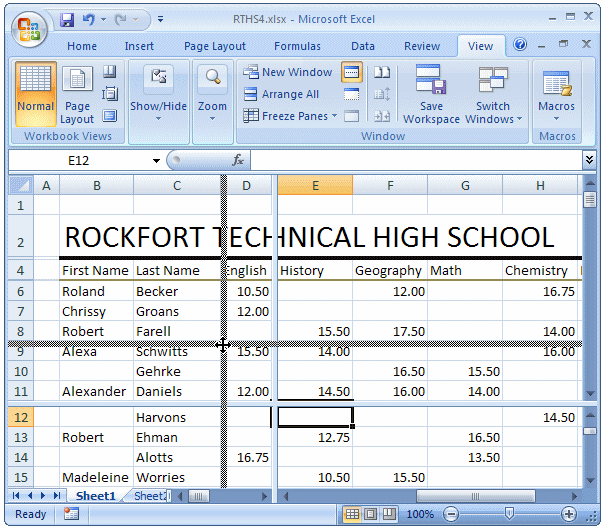
- Open the DAWN Report1.xlsx file
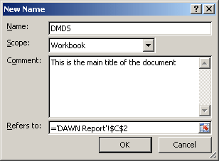
- To name a cell, click cell C2
- Click in the Name Box. That highlights C2. Type MainTitle and press
Enter

- Save the file
We already know how to select a group of cells. If you
select more than one cell, the name of the first cell displays in the Name Box.
In most operations, this cannot be useful, especially if you want to perform the
same operation on all cells in the selection. Fortunately, Microsoft Excel
allows you to specify a common name for the group of selected cells.
To specify a name for a group of cells:
- First select the cells as a group using the techniques we learned for selecting cells.
Then:
- In the
Name Box, replace the string with the new name
- On the Ribbon, click Formulas. In the Defined Names section, click
Define Name. In the Name text box of the New Name dialog box, type the desired name and
click OK
- Click any cell on the workbook:
- On the Ribbon, click Formulas. In the Defined Names section, click the
arrow of the Define Name button. In the New Name dialog box, in the Name text box, type the desired name.
In the Scope combo box, accept or specify the workbook. In the Comment
text box, type a few words of your choice if you want. In the Refers to
text box, click the button .
On the workbook, select the cells that will be part of the group. On the
New Name: Refers To dialog box, click the button .
Click OK
- On the Ribbon, click Formulas. In the Defined Names section, click
Name Manager. In the Name Manager dialog box, click New... In the Name text box, type the desired name.
In the Scope combo box, accept or specify the workbook. In the Comment
text box, type a few words of your choice if you want. In the Refers to
text box, click the button .
On the workbook, select the cells to include in a group. On the New
Name: Refers To dialog box, click the button .
Click OK. Click Close
|
Practical Learning: Naming Cells
|
|
- The DAWN Report1.xlsx file should still be opened.
Select cells A3:D16
- On the Ribbon, click Formulas. In the Defined Names section, click
Define Name
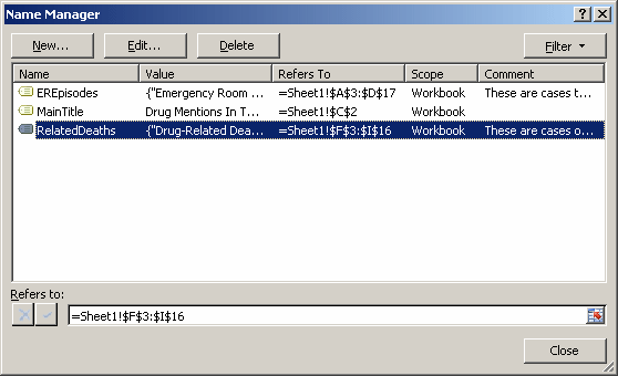
- In the Name text box of the New Name dialog box, type EREpisodes
- In the Comment section, type These are cases that brought a few patients to the emergency rooms at various hospitals in the country. The drug names refer to the types or categories of drugs that were consumed.
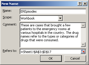
- Click OK

- Press Ctrl + Home
- In the Defined Names section of the Ribbon, click Name Manager...
- In the Name Name dialog box, click New...
- In the Name text box, type RelatedDeaths
- In the Comment text box, type: These are cases of deaths that occurred as a result of drug consumption or abuse.
- On the right side of the Refers to text box, click the selection
button
- Select cells F3:I16
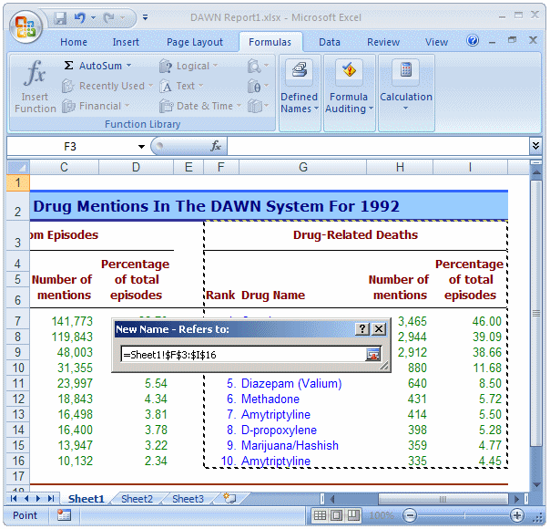
- On the New Name - Refers To dialog box, click the selection button
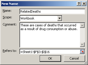
- Click OK
- On the Name Manager text box, click Close
- To review names, select cells A3:D16 and see the Name Box
- Select cells F3:D16

- Save and close the file
|
|