1. Start Microsoft Excel and open the Red Oak High School3 workbook.
   If necessary, click the ROSH worksheet to select it.
2. Select cells A1:C25
3. On the Formatting toolbar, click the arrow of the Fill Color button and select Pale Blue
4. Click column A to select it. Press and hold Ctrl, then click column C, and release Ctrl. That selects those two columns
5. Right-click column A and click Column Width…
6. Type 0.50 and click OK
7. Click cell B17 and type Red Oak High
8. Press Enter. In cell B18, type School
9. Press Enter. In cell B19, type Student Grade
10. Press Enter. In cell B20, type Book
11. Press Enter. In cell B21, type Mrs. Arlington
12. Press Enter. In cell B22, type The Student
13. Press Enter. In cell B23, type Administrator
14. Select cell B17:B23
15. On the Formatting toolbar, click the arrow of the Font Size combo box and select 8
16. On the same toolbar, click the Center button
17. Click the arrow of the Fill Color button and select Sky Blue
18. Click the arrow of the Font Color button and select White
19. While the cells are still selected, press Ctrl + 1 which is a shortcut for the Format Cells dialog.
20. In the Format Cells dialog, click the Borders property sheet. In the Line Style list, click the last line under None
21. Click the Color combo box and select White. In the Border section, click the top, the left, the right, and the bottom borders
     
    
22. Click OK.
23. Select cells B1:B25
24. On the main menu, click Format -> Cells to access the Format Cells dialog
25. In the Line Style section, click the 5th line on the second column
26. Click the Color combo box and select Teal
27. In the Border section, click the left and the right borders.
28. Click the Patterns property page. From the Cell Shading Color list, click Indigo (7th column, 1st row)
29. Click OK
30. Right-click column B and click Column Width
31. Type 9.50 and press Enter then press Ctrl + Home to see the result
     
    
32. Save the workbook

The Drawing Toolbar

The drawing in mainly done using the Drawing toolbar.

The Drawing toolbar is usually available on the bottom section of Microsoft Excel’s interface. If you don’t see it or to display and hide it anytime, right-click any button on any displayed toolbar. If Drawing has a check mark, this means that the Drawing toolbar is currently displaying on your screen. To hide it, you can click Drawing and the toolbar would disappear. If Drawing doesn’t have a check mark, you can then click it to reveal the Drawing toolbar. You can also get access to any toolbar by using the main menu where you would click View -> Toolbars, then proceed the same way as described above. Another way you can control the toolbars is from the main menu where you would click Tools -> Customize.

Although the Drawing toolbar is dockable, which means you can position it on the top, on the left, or on the right sides of your screen, it is better to keep at its default and usual position, which is at the bottom of your screen.

Practical Learning: Displaying the Drawing Toolbar

• To display the Drawing toolbar, on the main menu, click View -> Toolbars
  If the Drawing item has a check mark, then press Esc three times. If it doesn't, then click it

Shapes

A shape is an aesthetic figure you draw on a worksheet. There is no strict rule that defines what a shape looks like.

To draw a shape, click it on the Drawing toolbar, then on the worksheet, click one of the extreme end, drag to the other extreme, when you get a satisfying size and orientation, release the mouse. Once you release the mouse, the object will still be selected with various object handles of various sides and corners of the object. If you position your mouse on different handles or on the object, the mouse pointers will have different shapes.

Some objects don’t display all these mouse pointers and some may display different mouse shapes. If/when one of those unusual pointers comes up, you will be guided on its meaning.

Almost any shape you draw has a marking rectangular box around it. This allows you to work on the shape as an object. For example, you can use this box to move the object.
You can move any object to a new location on your screen. Sometimes you will want to select more than one object to manipulate the group. To select more than one object, click one of them, press and hold Shift, and click the other object(s). When you have created the group, release Shift.

A drawn object can be copied and pasted to another location on the same worksheet or to a different worksheet on the same workbook, in another workbook, or even to another file. To copy an object, click it. Then on the main menu, click Edit -> Copy, and proceed with pasting. You can copy one object or a group of objects. Using the new Clipboard toolbar of Microsoft Office 2000, you can copy up to 12 objects at once, then paste them to their new respective locations. Just keep in mind that these objects will not have explicit names.

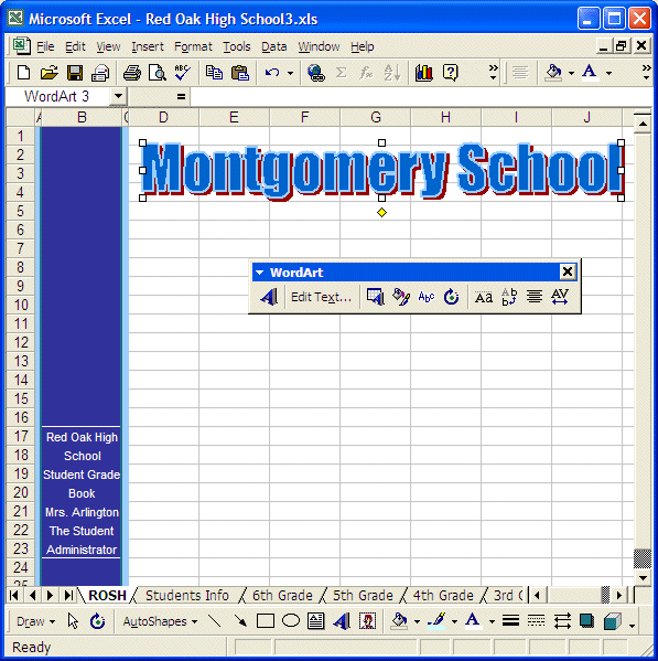
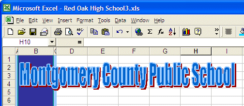
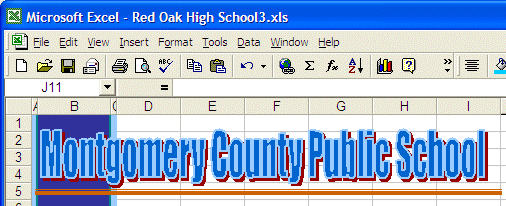
Microsoft Office WordArt

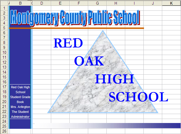
A Microsoft Office WordArt is a fancy formatted sentence whose features you can use to include a good-looking group of words that you type and embed in your worksheet.
To get a WordArt, you can click the Insert WordArt button on the Drawing toolbar. From the WordArt Gallery dialog, select the style you like and click OK. Type the desired sentence; you can also change the font and/or font size before clicking OK. Once the WordArt has been created, you can move and resize it to your satisfaction.

Whenever the WordArt is selected, the WordArt toolbar should be on your screen, this toolbar is very useful and you should always have it handy whenever you are working on a WordArt.
Even after the WordArt has been created, you can change its wording and style. To control its text, when the WordArt is selected, double-click or right-click it and click Edit Text, rephrase the words and click OK. To change the WordArt style, click the WordArt Gallery button the WordArt toolbar, select a new style and click OK.

Practical Learning: Creating WordArt

1. On the Drawing toolbar, click the Insert WordArt button
2. Click the WordArt on 5th column, 2nd row
    
   
3. Click OK
4. Change the Size combo box to 20
5. Replace the text with Montgomery School and click OK
6. While the WordArt is selected, resize and move it to occupy the upper section of the screen
    
   
7. On the WordArt toolbar, click the Edit Text… button.
8. Click between both words and type County Public so that when you finish, the text will read Montgomery County Public School
    
   
9. Click OK
10. On the WordArt toolbar, click the WordArt Gallery button
11. Click the WordArt on 2nd column, 2nd row
12. Click OK
13. Press Ctrl + Z to undo
14. Resize and re-position the title as you see fit but somewhere in the top-left section of the worksheet
     
    
15. Save the workbook

Drawing Lines

One of the shapes available to improve your worksheet is the line. You can draw a horizontal, vertical, or diagonal line. When drawing lines, you can control their width, color, and arrow orientation if you decide to be fancy.

To draw a line, click it on the Drawing toolbar. Then, on your worksheet, click one of the line’s intended starting points and drag on the other side, when you get the desired length or orientation, release the mouse. To draw a line starting at its center, press and hold Ctrl while you are dragging. To draw a controllable line, for example horizontal or vertical, press and hold Shift while you are dragging.

When you have just released the mouse, the drawn line is terminated by small boxes on both sides. Use these object handles to control the line’s size and orientation.

Practical Learning: Drawing and Controlling Lines

1. On the Drawing toolbar, click the Line button.
2. To draw a horizontal line, press and hold Shift. Click around the left border of cell B5 and hold your mouse down. That marks the starting point of our line.
3. Drag the mouse in the right direction until you get to the right border of cell I5, then release the mouse. You don’t have to be absolutely precise since you can still resize and move the line to meet your satisfaction.
4. While the line is still selected, on the Drawing toolbar, click the arrow of the Line Color button and click More Line Colors…
5. From the Colors dialog, click the Custom property page
6. Change the values of the colors to Red: 204, Green: 102, Blue: 0. Click OK
7. On the Drawing toolbar, click the Line Style button and select the 3rd line from bottom (4 ½ pt)

Microsoft Office Drawing Shapes

The Drawing toolbar is equipped with numerous shapes, some of which you are familiar with, and you will get acquainted with some others. The drawing shapes on the Drawing toolbar are essentially organized in two categories. The most classic ones are readily on the toolbar; these are the Line, the Arrow, the Rectangle, and the Oval. The Line is just used to draw familiar lines. The Arrow is used to draw fancy lines terminated on one side or on both with an arrow or a bullet. The Rectangle is used to draw a rectangle or a square (a four-sided geometric figure whose sides are all equal).

To draw a regular rectangle, click the Rectangle button. On the worksheet, click one intended corner of the rectangle and hold your mouse down. Drag to the other end corner of the rectangle and release the mouse. When you get the size you want, release the mouse. If the size and the position are not satisfying, you can resize and move the rectangle to your liking, using the rectangle’s handles. To draw a rectangle starting at its center instead of its corner, press and hold Ctrl while you are dragging. To draw a rectangle starting at the corner of a cell, press and hold Alt while you are dragging.

To draw a square, press and hold Shift while you are dragging. To draw a square starting at its center instead of its corner, press and hold Ctrl + Shift while you are dragging. To draw a square starting at the corner of a cell, press and hold Shift + Alt while you are dragging.

The Oval is used to draw an ellipse or a circle. Apply the techniques we have reviewed for the rectangle, just keep in mind that this time, the shape is circled.

Other drawing shapes are available from the AutoShapes on the Drawing toolbar; these are organized in sub-categories of Lines, Basic Shapes, Block Arrows, etc.

Practical Learning: Drawing Shapes

1. Click the Student Info sheet to make it active
2. On the Drawing toolbar, click AutoShapes -> Basic Shapes -> Octagon
3. On the worksheet, click on the left side of cell A7
4. Resize the shape to fit the dark gray area
5. While the shape is still selected, on the Drawing toolbar, click the arrow of the Fill Color button and click Fill Effects…
6. In the Fill Effects dialog box, make sure you are in the Gradient property page. In the Shading Styles section, click From Center
7. In the Variants section, make sure that the first button (1st column, 1st row) is selected Click OK.
8. On the Drawing toolbar, click the arrow of the Line Color button, and click No Line
9. On the Drawing toolbar, click the Rectangle button
10. Click above the letter R of the RED OAK title in the upper section of the worksheet
     
    
11. Type RED OAK HIGH SCHOOL 
12. Select the new typed words in the rectangle
13. On the Formatting toolbar, change the Font to Garamond and the Font Size to 20, also click the Bold button
14. Resize the rectangle to display all the typed words
15. Right-click the border of the rectangle and click Format AutoShape
16. From the Format AutoShapes dialog box, click the Font property page, change the Color to White
17. Click the Alignment property page
18. In the Text Alignment section, change the Horizontal and the Vertical combo boxes to Center each
19. Click the Colors And Lines property page
20. In the Fill section, click the Color combo box and select No Fill
21. In the Line section, click the Color combo box and select Light Yellow (3rd column, 5th row)
22. In the Dashed combo box, make sure that the Solid (continuous) line is selected, decrease the line Weight spin button to 0.5 pt
23. Click the Size property page
24. In the Size And Rotate section, set the Height spin button to 0.4”
25. In the Width spin button, type 3.54 and press Tab. Make sure the Rotation spin button is set to 0°. 
     
    
26. Click OK
27. On the Drawing toolbar, click AutoShapes -> Basic Shapes -> Rounded Rectangle
28. Draw and size a shape that completely covers the former shape, the RED OAK HIGH SCHOOL title
29. While the shape is still selected, on the Drawing toolbar, click the arrow of the Fill Color button and click Fill Effects…
30. In the Fill Effects dialog, click the Texture property page
31. In the Texture list, click Brown Marble (3rd column, 2nd row). Click OK
32. On the Drawing toolbar, click the arrow of the Line Color, and select White
33. On the Drawing toolbar, click the Line Style button, and click 1 pt
34. While the shape is still selected, on the Drawing toolbar, click Draw -> Order -> Send Backward. Now both shapes should be visible
35. While one of the shapes is still selected, press and hold Shift, click the other shape (the rectangle with RED OAK), and release Shift when both shapes have been selected
36. On the Drawing toolbar, click Draw -> Align Or Distribute -> Align Center
37. While the shapes are still selected, move the whole group so that the left border of the brown marble aligns with the left border of column B
38. Click somewhere else to deselect the shapes. Press Ctrl + Home
     
    
39. Click the ROSH Cover worksheet to select it
40. Click the lower right border of the triangle to select its shape
41. Press and hold Shift, click RED on the big text, click the wide rectangle at the bottom section of the screen, then release Shift. That selects these three shapes
42. On the main menu, click Edit -> Copy
43. Click the ROSH worksheet to make it active
44. On the main menu, click Edit -> Paste
45. While the shapes are still selected, move them on the top section
46. Click somewhere else to deselect and press Ctrl + Home

ClipArt and Pictures

Microsoft Office ships with a lot of pictures that you can use to enhance your worksheet. You can also include almost any kind of picture from almost any format.

The ClipArt Gallery that installs with Microsoft Excel organizes its files in various categories. To access them, on the main menu, you can click Insert -> Picture > ClipArt. Select a category by clicking its button, review the available picture, once you like one, click it, and click Insert from the menu that comes up. You can also access additional pictures from Microsoft web site.
Using any commercial graphics software, you can also create your own graphics. You can as well use company or personal pictures. Once you have one of these pictures or images in a suitable electronic format, on the main menu, click Insert -> Picture -> From File… Locate the folder where the picture is located, and select it.

Microsoft Excel also allows you to completely change a worksheet’s background with a picture of your choice.

Practical Learning: Including Microsoft Office ClipArt

1. On the main menu, click Insert -> Picture -> ClipArt…
2. From the Insert ClipArt dialog, click Animals. Click the Lion (1st column, 1st row) and click Insert Clip
3. Close the ClipArt dialog box
4. Using its lower right handle, resize the picture to occupy the Pale Blue section from the left corner of cell B6 to the lower right corner of cell B6
5. On the main menu, click Format -> Sheet -> Background…
6. From your Exercises folder, click roshbg1 and click OK.
7. On the main menu, click Tools -> Options…
8. Make sure you are in the View property page. In the Window section, uncheck the Gridlines check box. Click OK
9. Save your workbook