Worksheets Fundamentals

As you may realize, Microsoft Excel's primary purpose is to help you create lists using readily available cells spread on a sheet that resembles a piece of paper. For this reason, Microsoft Excel is referred to as a spreadsheet application. In Microsoft Excel, the list of cells of a document is called a worksheet.

Even when they belong to the same document, worksheets can be treated as independent entities, although it is more suitable that they be treated as a unit.

In some circumstances, you will need to perform a general action on a worksheet. Before doing this, you may need to select the contents of the whole worksheet first. Since there are usually many worksheets presented to you, each is represented by a tab on the lower left corner. Therefore, to select a worksheet:

• You can click its tab
• You can press and hold Ctrl. Then press either Page Up or Page Down. Once the desired worksheet has been selected, you can release Ctrl

If you have many worksheets, to select a range of worksheets, click a tab that is considered one end of the range. Press and hold Shift, then click the tab at the end of the range and release Shift.

To select worksheets at random, click one of the desired worksheets. Press and hold Ctrl. Then click each desired worksheet. When the selection has been made, release Ctrl.

1. Open the Grier Summer Camp1 workbook
2. To select a worksheet, in the lower left corner, click Sheet3
    
   
3. To select another worksheet, click Sheet2
4. Press and hold Ctrl
5. Press Page Up. Notice that you are switched to Sheet1
6. Press Page Down
7. While you are still holding Ctrl, press Page Up. Notice that you are now in Sheet1
8. Release Ctrl
9. Click Sheet1 if necessary.
   To select more than one worksheet, press and hold Ctrl and Shift
10. Press Page Down once. Notice that Sheet1 and Sheet2 have been selected
     
    
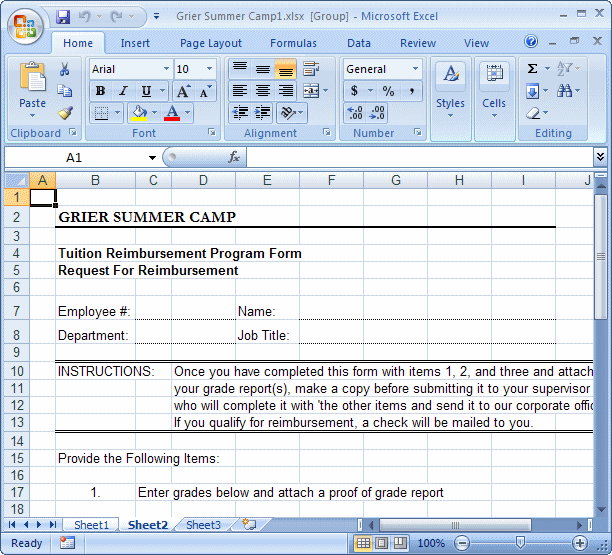
11. Press Page Down again to select three worksheets
12. Release Ctrl and Shift then click Sheet1

The starting worksheets are named Sheet1, Sheet2, and Sheet3. You can change any or all of these worksheet names.

To rename a worksheet:

• You can double-click its sheet tab, then type a new name
• You can right-click a sheet’s tab, click Rename, and type the new name
• While a certain worksheet is selected, on the Ribbon, click Home. In the Cells section, click Format. In the Organize Sheets section, click Rename Sheet:
   
  
  
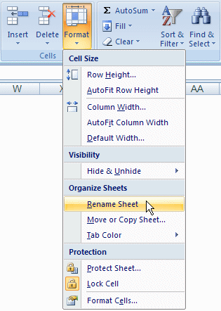
  Then type the new name, and press Enter

1. To rename the first worksheet, double-click the Sheet1 tab to put it in edit mode
2. Type Request For Time Off
3. To rename the second worksheet, right-click the Sheet2 tab and click Rename from the shortcut menu
4. Type Tuition Reimbursement
5. To rename the third worksheet, click Sheet3 to make it the active worksheet
6. On the Ribbon, click Home if necessary.
   In the Cells section, click Format and click Rename Sheet
7. Type Time Sheet and press Enter
    
   
8. Save the document

To show the limits of a cell, it displays borders around it. These borders are also referred to as gridlines. If you want, you can show or hide the gridlines.

To hide the gridlines of cells of a worksheet, on the Ribbon:

• Click Page Layout. In the Sheet Options section, under Gridlines, remove the check mark on View:

• Click View. In the Show/Hide section, remove the check mark on the Gridlines check box

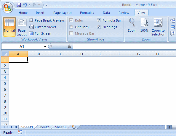
To show the gridlines again:

• In the Sheet Options section of the Page Layout tab of the Ribbon, under Gridlines, put a check mark on the View check box
• In the Show/Hide section, of the View of the Ribbon, click the Gridlines check box

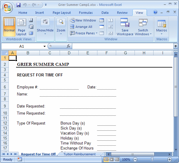
1. Click the Request For Time Off tab
2. On the Ribbon, click View
3. In the Show/Hide section, click the Gridlines check box to uncheck it
    
   
4. Click the Tuition Reimbursement tab
5. Press and hold Ctrl
6. Click the Time Sheet tab
7. On the Ribbon, click Page Layout
8. In the Sheet Options section, under Gridlines, click the View check box
9. Save the file

We were introduced to columns in Lesson 2 and to rows in Lesson 3. We also saw the columns start in the top section by column headers and the rows start on the left by row headers. The column headers and the row headers are characteristics of a worksheet. This means that you can show or hide the column headers or the row headers for a worksheet while the headers are hidden or shown for another worksheet.

By default, the column headers and the row headers display on their worksheet. To hide the headers:

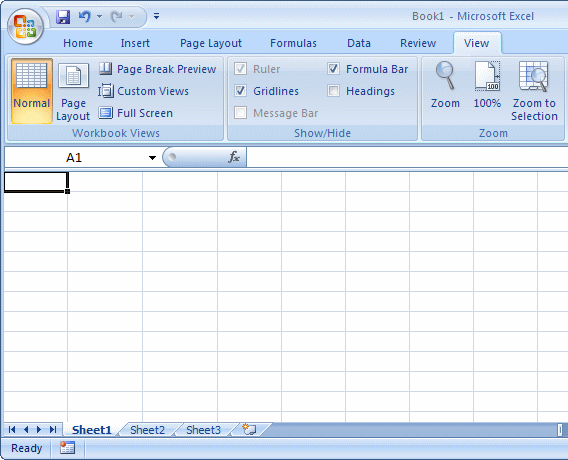
• On the Ribbon, click View. In the Show/Hide section, remove the check mark on the Headings check box:

• Click Page Layout. In the Sheet Options section, under Headings, remove the check mark on View:

To show the headers again:

• In the Show/Hide section, of the View tab of the Ribbon, click the Headings check box
• In the  the Sheet Options section of the Page Layout tab of the Ribbon, click the Headings check box

1. Click the Request For Time Off tab
2. Press and hold Shift
3. Click the Time Sheet tab
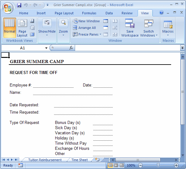
4. On the Ribbon, click View
5. In the Show/Hide section, click the Headings check box to uncheck it
    
   
6. Click the Tuition Reimbursement tab
7. Click the Request For Time Off tab
8. Save the file

The regular view of a worksheet is referred to as normal. It shows one large and long display of columns and cells. Microsoft Access allows you to choose among many other views.

Instead of the regular or normal view, to change how a worksheet displays its cells, on the Ribbon, click View and click one of the buttons in the Workbook View section:

• Normal: This is the regular view of a worksheet
• Page Layout: This would divide the cells into various groups depending on the width of the cells on the worksheet:

• Page Break Preview: This view shows how the pages would be printed by dividing the worksheet in page breaks:

• Full Screen: The worksheet would use the whole screen

To get the regular view from Page Layout or Page Break Preview, you can click the Normal button. To get the normal view from Full Screen, you can press Esc.

By default, worksheets are positioned in a numbered format that makes it easy to count them. More often you will find that, after creating a few of them, you are not satisfied with their positions. You should be able to reposition them in a manner that suits your particular scenario.

To move a worksheet, click and hold the mouse on its tab, then move the mouse in the direction of your choice. While you are moving the worksheet, the mouse pointer will turn into a white piece of paper and a small down-pointing triangle will guide you. Once the small triangle is positioned in the desired location, release the mouse.

1. Click and hold the mouse on the Request For Time Off tab
2. Move the mouse in the right direction. Notice that the mouse pointer turns into a white piece of paper and there is a small triangle that guides you
3. Once the small triangle is positioned between Tuition Reimbursement and Time Sheet, release the mouse
    
   
4. Now we will move the Time Sheet worksheet because that is the form that employees are using on a regular basis before anything else.
   Click the hold the mouse on the Time Sheet tab
5. Move the mouse in the left direction
6. When the small triangle is positioned to the left of Tuition Reimbursement, release the mouse
7. Save the file

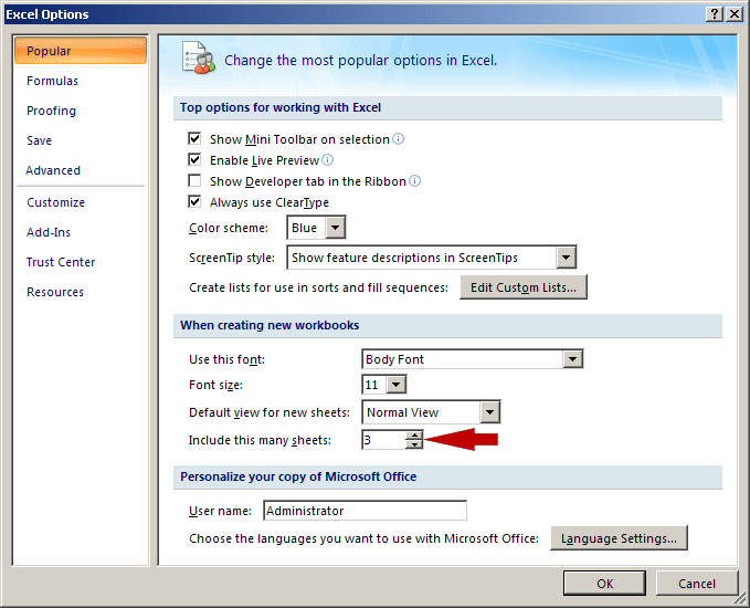
As mentioned already, when Microsoft Excel starts, by default, creates three worksheets. We also mentioned that you can change this default number in the Excel Options dialog box. You can add a new worksheet anytime if you judge it necessary.

Some workbooks are quite complete with just one worksheet, but others need as many worksheets as possible. The number of worksheets you use in a particular workbook is conditioned by your needs and the memory of your computer.

To add a new worksheet to a workbook:

• Click the small tab on the right side of the existing tabs
   
  
• Click the worksheet tab that will succeed the new worksheet and press Shift + F11
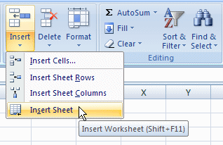
• On the Ribbon, click Home. In the Cells section, click the arrow under the Insert button and click Insert Sheet
   
  
• Right-click a sheet tab and click Insert... This would display the Insert dialog box:
   
  
  
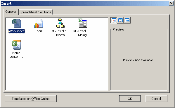
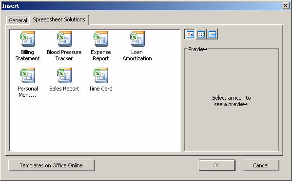
  From the Insert dialog box, you can choose to insert a blank worksheet or insert one of the existing templates as a worksheet:
   
  

1. To start a new workbook, press Ctrl + N
2. On the Ribbon, click Home if necessary. In the Cells section, click Format and click Rename Sheet 
3. Type Students Info
4. Double-click the Sheet2 tab to highlight it
5. Type Emergency Information
6. Right-click the Sheet3 tab and click Rename
7. Type 6th Grade and press Enter
8. Right-click the 6th Grade tab and click Insert…
9. In the Insert dialog, make sure that the General property page is selected; if it is not, click it and click Worksheet
    
   
10. Click OK
11. Right-click the new Sheet4 tab and click Rename
12. Type 5th Grade and press Enter
13. In the Cells section of the ribbon, click the down-pointing button under Insert and click Insert Sheet
14. To change the name of the current worksheet, in the Cells section of the Ribbon, click Format -> Rename Sheet 
15. Type 4th Grade and press Enter
16. Press Shift + F11
17. Double-click the new Sheet tab to highlight it
18. Type 3rd Grade and press Enter
19. Press F4 to add a new worksheet
20. Double-click the new sheet tab to rename it
21. Type 2nd Grade and press Enter
22. Press Shift + F11 to insert another worksheet
23. Right-click the new sheet tab and click Rename
24. Type 1st Grade and press Enter
25. Press F12 to save the workbook
26. Set its name to Solstice Academy1 and press Enter

As your work progresses, you will decide how many worksheets you need for your particular workbook. Just as we learned to add worksheets, you can delete or remove the worksheets you don't need anymore. Since a worksheet is not a file, when you delete a worksheet, it is permanently gone. If one or more cells of the worksheet contain data, you will receive a confirmation message to decide.

To delete a workbook:

• You can right-click its tab and click Delete
• In the Cells section of the Home tab of the Ribbon, click the arrow of the Delete button and click Delete Sheet

1. To delete a worksheet, right-click the Emergency Information tab and click Delete
2. Move and arrange the worksheet so that from left to right you will have Student Info, 6th Grade, 5th Grade, 4th Grade, 3rd Grade, 2nd Grade, and 1st Grade
3. Save the file

As mentioned already, by default, Microsoft Excel makes three worksheets available to you. We also reviewed how you can add new ones or delete some of them. Instead of deleting a worksheet, you can hide it for any reason you judge necessary. If the workbook contains more than one worksheet, you can hide one or more worksheets or even the entire workbook.

To hide a worksheet in a workbook, click any cell in that worksheet to make it active:

• Right-click the sheet tab and click Hide
• In the Cells section of the Home tab of the Ribbon, click Format, position the mouse on Hide & Unhide, and click Hide Sheet
   
  

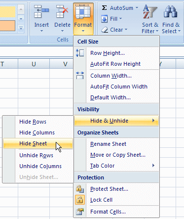
The worksheet’s tab will disappear from the screen although it is not deleted. To hide a group of worksheets, select them and proceed in the same way. 

To unhide the hidden worksheets:

• Right-click any tab and click Unhide...
• In the Cells section of the Ribbon, click Format, position the mouse on Hide & Unhide, and click Unhide Sheet...

This would open the Unhide dialog box with a list of the the names of the hidden worksheets:

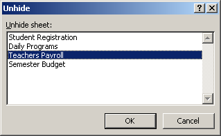
If you have more than one hidden sheet, select the desired worksheet and click OK.

1. Right-click the Student Info tab and click Hide
2. Click the 3rd Grade tab
3. Press and hold Ctrl
4. Click the 1st Grade tab
5. On the Ribbon, click Home if necessary.
   In the Cells section, click Format, position the mouse on Hide & Unhide, and click Hide Sheet
    
   
6. To unhide the worksheets, right-click any sheet tab and click Unhide...
7. In the Unhide dialog box, click 1st Grade and click OK
8. In the Cells section of the Ribbon, click Format, position the mouse on Hide & Unhide, and click Unhide Sheet...
9. In the Unhide dialog box, click 3rd Grade and click OK
10. Right-click any sheet tab and click Unhide...
11. In the Unhide dialog box, click OK
12. Close Microsoft Excel. If asked whether you want to save, click No

You can publish the content of a worksheet to a web page. In Microsoft Excel, you can publish just one worksheet or the whole workbook. To perform publishing, first decide on what you want to publish, a worksheet or the whole workbook.

To save a file for the web, click the Office Button, position the mouse on Save As and click Other Formats. In the Save As Type combo box, select Web Page (.html). Specify whether to save the whole document or only some worksheets. Click Save. Read the message box and click Yes.