|
In Lesson 3, we saw that, when Microsoft
Excel starts, it creates 16,384 columns. In Lesson 4, we saw that when Microsoft
Excel starts, it creates 1,048,576 rows. As a result, when you open Microsoft
Excel, you have a total of 16,384 * 1,048,576 = 17,179,869,184 cells available. You can use just a few of them, as will usually be the case, or you
can use as many as you want but they are always available.
Among the various ways you can use a cell, we will see in
various sections that you can click it or use the keyboard to get to a cell. You
can also right-click a cell. When you do, a multi-part menu would appear:

Notice that the context-sensitive menu is divided in two
sections; a toolbar and a menu window. Throughout our lessons, we will see what
the buttons and the menu items represent.
Whatever you are doing on a cell, it is always
important to know what cell you are working on. The minimum piece of
information you need about a cell is to know which one you are using at a
particular time. To make this recognition a little easier, each cell has
an address also called a location. This address or location also serves as the
cell's primary name.
To know the location of a cell, you refer to its
column and its row. The combination of the column's name and the row's
label
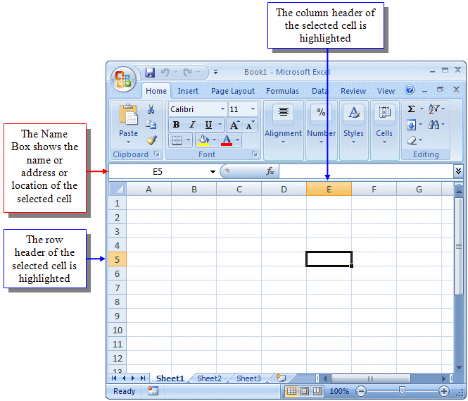
provides the address or name of a cell. When you click a cell, its column header
becomes highlighted in orange. In the
same way, the row header of a selected cell is highlighted in orange. To know the name of a cell, you can refer to the Name Box, which
is located at the intersection of columns and rows' headers:
|
 Practical
Learning: Identifying a Cell Practical
Learning: Identifying a Cell
|
|
- Open the RTHS4.xlsx file
- Click any cell in the document and notice its name in the Name Box
- Press Ctrl + Home
Before doing anything on a cell or a group of cells,
you must first select it. Selecting cells is almost equivalent to highlighting
a word in a text document. Various means are available to select a cell or
a group of cells. You can use the mouse only, the keyboard only, or a
combination of the mouse and keyboard.
At almost any time, at least one particular cell is selected.
The selected cell has thicker borders than the other cells. That cell is
referred to as the active cell. This is important because you always need to know where the changes you are making are being applied. This means
that, whatever you type or format will apply to that particular cell. Sometimes you will want to work on many cells simultaneously. Therefore, you first have to select the intended cells before proceeding.
As mentioned already, you can select a cell using the
mouse, the keyboard, or a combination:
- To select a cell using the mouse, just click it. To select another cell, click the new
one
- To select a cell using the keyboard, since you may have to move focus from
one active cell to another, press the arrow keys until the desired cell is
selected
- To select a cell based on its name and using the mouse and keyboard, click
in the Name Box, and type the name or address of the cell
- To select the first cell of the document using the keyboard only, press
Ctrl + Home
|
 Practical Learning: Selecting Cells Practical Learning: Selecting Cells
|
|
- To select one cell at a time, click cell B6
- Click cell C4
- Click cell E8
- Press the down arrow key
- Press the right arrow key three times
- Press Ctrl + Home
Instead of only one cell, you may want to perform a
common operation on many cells, which means you must select them first.
You can use the mouse, the keyboard, or a combination. You can select
cells based on columns or based on rows. You can select cells in a
particular region; that is, adjacent cells, or you can select non-adjacent
cells:
- To select all cells of a column:
- Click the column header
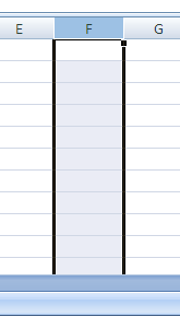
- In the Name box, type the name of a cell of that column and press
Enter. Then press Ctrl and the Space bar
- To select all cells of a series of columns, select those columns as seen
in Lesson 2 and notice that all cells in the selected columns are selected
- To select all cells of a row:
- Click the row header as seen in Lesson 3
- In the Name box, type the name of a cell of that row and press Enter.
Then press Shift and the Space bar
- To select all cells of a series of rows, select those
rows as seen in Lesson 3 and notice that all cells on the right side of the
selected rows are highlighted
- To select cells in the same region using the mouse only, click and hold your mouse on one cell, then drag down
or up, left or right, to the last cell in the range
- To select cells in the same region using the keyboard only, press the
arrow keys a few times until the cell that will be at one corner is
selected. Press and hold Shift. Press the arrow keys left, right, up, or
down.
If you press the right
arrow key, the currently highlighted cell and the cell to its right
would be selected. If you press the down arrow key, the current cell and the cell under it will be highlighted. You can also press the left or up arrow
key. You can press the arrow keys many times in the direction of your choice. Once you have achieved the selection you want, release the Shift
key
- To select non-adjacent cells, click one of the cells. Press and hold Ctrl.
Click each of the desired cells. Once the selection is complete, release
Ctrl
- To
select all cells on a worksheet, you can press Ctrl + A. Alternatively,
you can click the button at the intersection of the row header and row
headers
|
 Practical Learning: Selecting Cells Practical Learning: Selecting Cells
|
|
- To select multiple cells on the same column, click Column Header C
- To select multiple cells on the same row, click Row Header 15
- To select cells in a range, click and hold the mouse on cell B8, your mouse turns into a big + sign
- Drag the mouse in the right direction until 17.50 in cell F8 is selected, then release the mouse. Notice that
5 cells are selected

- Click Cell C7
- Press and hold Shift
- Then click Cell C15 and release Shift

- Click cell C7 and hold the mouse down
- Drag the mouse right and down
to cell E11 to include it in the highlighted
range
- Release the mouse. That selects adjacent cells in the same area

- Click Cell B6
- Press and hold Shift
- Press the down arrow key twice
- Press the right arrow key 4 times
- Release Shift
- Press Ctrl + Home
- To select cells at random, click cell D9. Press and hold Ctrl. While you are holding Ctrl, click cells B7,
H12, and E15
- Release Ctrl

- Press Ctrl + Home
- To select all cells, click the button on the intersection of the row
and row
headers

- To deselect, click cell C4
- Press Ctrl + Home
|
 From now on, unless specified otherwise, the following conventions will be used
|
| Instruction |
Means |
| Click G5 |
Click
cell G5 |
| Select B2:F8 |
Select
cells from B2 to F8, and that will include all cells in the range B2
to F8 |
| Select cells D4, B10, A2, and H16 |
Select only those cells at random |
| Click cell F4 |
Using
your mouse, click cell F4. On the other hand, if I write press
F4, I mean using your keyboard, press function
key F4. Remember that "click" refers to using the mouse and
"press"
refers to using the keyboard |
| Select row 4 |
Position
the mouse on the row header which is the gray box where the row number is
displaying, then click |
| Select rows 4 and 5 |
Use one of the methods we learned to select the row headers |
| Select
rows 4:8 |
Use one of the methods we learned to select the row headers |
| Select row E |
Position
the mouse on the row header which is the gray box where the row letter(s) is displaying, then click |
| Select rows D and F |
Use one of the methods we learned to select the row headers |
| Select rows C:H |
Use one of the methods we learned to select the row headers |
A cell uses a combination of the width of its parent
column and the height of its parent role to determine its size. This means
that the width of a cell is the width of its column and its height is that
of its row. Therefore, to change or specify the size of a cell, you use
the technique of setting the width of columns or the height of cells as we
saw in Lessons 3 and 4.
|
Controlling the Widths of Cells
|
|
In future lessons, we will see how to enter values in
cells. We will find out that it is not unusual that the content of a cell
goes beyond its normal size. To show the hidden content of a cell, you can
resize it.
As seen in Lesson 2:
- To control the width of all cells of a column, position the mouse on the
separating line between two column headers. Drag left or right until
you get the desire width. Then release the mouse.
- To change the widths of cells of a group of columns, first select the columns,
whether in a range or randomly. Position the mouse on the column header border of one of the selected
columns. Click and drag left or right in the direction of your choice until
you get the desired with. Then release the mouse.
- If a cell under a column header displays the width
you want,
click the box that has the desired width. Then:
- Double-click the
separating
line between the column header
- On the Ribbon, click Home. In the Cells section, click Format and click
AutoFit Column Width
- If many columns have some cells width a desired width, select those cells as
we saw earlier. Then:
- Double-click the separating line on one side of the column headers
- On the Ribbon, click Home. In the Cells section, click Format and click
AutoFit Column Width
- To precisely set the width of cells under a column:
- Right-click the column header and click Column Width...
- Click a column header or any of its cells. On the Ribbon, click
Home. In the Cells section, click Format and click Column Width...
- To specify the same width for many columns:
- Select a range of columns. Right-click
either one of the column headers or inside the selection and click Column
Width...
- Randomly select a group of (non-adjacent) columns. Right-click one of the
column headers and click Column Width...
- Select the columns, whether in a range or randomly (non-adjacent). On the
Ribbon, click Home. In the Cells section, click Format and click Column
Width...
Any of these actions would
open the Column Width dialog box. From there, accept or enter the desired value
and click OK
To undo any of these actions:
- On the Quick Access toolbar, click the Undo button

- Press Ctrl + Z
|
 Practical Learning:
Setting the Widths of Cells Practical Learning:
Setting the Widths of Cells
|
|
- Click Cell D4 to select it
- On the Ribbon, click Home if necessary.
In the Cells section, click Format and click
AutoFit Column Width
- Select Cells E4:I4
- In the Cells section of the Ribbon, click Format and click Column
Width...
- Type 10 and click OK
- Press Ctrl + Home
|
Controlling the Heights of Cells
|
|
In Lesson 3, we saw different techniques of setting or
controlling the heights of rows. Actually, these apply to cells on the right
side of the rows. As a reminder:
- To change the height of the cells of a row, click
the lower border of a row header. Drag up or down until you get the desired
height. Then release the mouse
- To change the height of cells on the right sides of a group of rows, first select the
rows. Position the mouse on the bottom border of one of the selected rows. Click and drag
up or down in the direction of your choice until
you get the desired height. Then release the mouse.
- If the cells on the right side of a row header are too short or too tall,
to change their height:
- Double-click the bottom border of the row header
- Click the row header. On the Ribbon, click Home. In the Cells section, click Format and click
AutoFit Row Height
- To precisely specify the height of cells of a row:
- Right-click the row header and click Row Height...
- Click a row header or any box on its right side. Then, on the Ribbon, click
Home. In the Cells section, click Format and click Row Height...
- To precisely set the same height for cells of many rows:
- Select a range of rows. Right-click either one of the
row headers or inside the selection and click Row Height...
- Randomly select a group of (non-adjacent) rows. Right-click one of the row
headers and click Row Height...
- Select the rows. On the
Ribbon, click Home. In the Cells section, click Format and click Row
Height...
This would call the Row Height dialog box where you can type the desired value
and click OK or press Enter
To undo any of these actions:
- On the Quick Access toolbar, click the Undo button

- Press Ctrl + Z
|
Creating Cells Vertically
|
|
As mentioned already, when Microsoft Excel starts, it
creates billions of cells for you. As we will see in the next lessons, you can
then use the cells to enter the values you want in your spreadsheet. As a list
displays its values, you may want to insert a value between two existing cells.
In Lesson 2, we saw that you could insert a new column to
get new cells on the left side of a series of existing cells. Instead of using
the column to perform this operation, you can do it from inside the cells.
To add a new column:
- Right-click a cell that belongs to the column that will follow the new
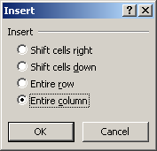
column and click Insert... This would open the Insert dialog box. To insert a new column, click the
Entire Column radio button before clicking OK:
- Click a cell. On the Ribbon, click Home. In the Cells section, click the arrow
button under Insert and click Insert
Sheet Columns
- Click a cell. On the Ribbon, click Home. In the Cells section, click the arrow under Insert and click Insert
Cells... This would open the Insert dialog box. To insert a new column,
click the Entire Column radio button and click OK
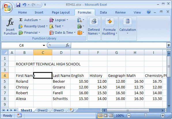
When you perform any of these operations, a new column would
be created on the left side of the column whose cell was clicked or right-clicked:
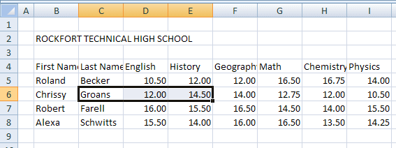
To add more than one column, first select the cells, either in a
range:
Or at random:
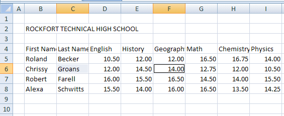
Then:
- Right-click one of the selected cells and click Insert... In the Insert dialog
box,
click the Entire Column radio button and click OK
- Click a cell. On the Ribbon, click Home. In the Cells section, click the arrow under Insert and click Insert
Sheet Columns
- Click a cell. On the Ribbon, click Home. In the Cells section, click the arrow under Insert and click Insert
Cells... This would open the Insert dialog box. To insert a new column,
click the Entire Column radio button and click OK
When you perform one of these actions, if the cells were
selected in a range, the same number of columns would be created on the left
side of the range that was selected. If the selected cells where not adjacent,
new columns would be created on the left side of the column of each cell that
was selected or on the left side of each group of cells that were selected.
The techniques of inserting columns that we saw in Lesson 2
and above are used to add a complete column. Sometimes, you will want to create,
add, or insert a new cell between two existing cells. To perform this operation
vertically, you would ask Microsoft Excel to consider a cell, move all cells
under it by one step down. Once this is done, you would be presented with a new
empty cell where the other was.
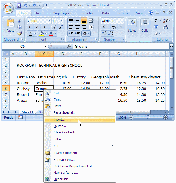
To insert a cell vertically between two cells:
- Right-click the cell that will be pushed down along with the cells under
it, and click Insert...
- Click the cell that will be pushed down along with its bottom neighbors.
On the ribbon, click Home. In the Cells section, click the arrow button
under Insert, and click Insert Cells...
Any of these actions would call the Insert dialog box. From
it, to insert a cell and push the other cells down, click the Shift Cells Down
radio button:
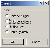
When you click OK, each cell would be pushed down up to the
cell that must be created:
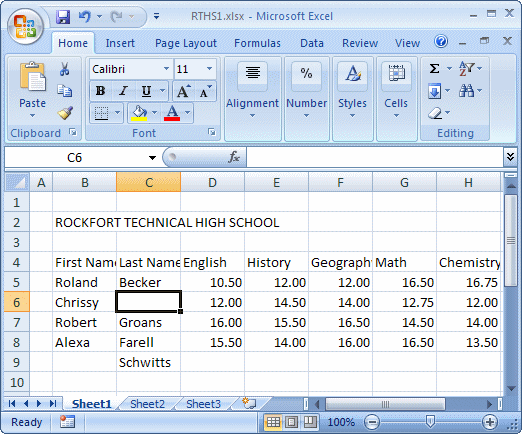
In the same way, you can first select cells in a column,
either in a range or randomly, and insert new cells.
To undo any of these actions:
- On the Quick Access toolbar, click the Undo button

- Press Ctrl + Z
|
Creating Cells Horizontally
|
|
In Lesson 3, we saw that you could add a new row to
get a new series of cells aligned horizontally. Those operations can also be
performed from cells.
To add a new row:
- Right-click a cell that belongs to the row that will be below the new row and click
Insert... This would open the Insert dialog box. To insert a new row, click the
Entire Row radio button and click OK
- Click a cell. On the Ribbon, click Home. In the Cells section, click the arrow
button under Insert and click Insert
Sheet Sheet Rows
- Click a cell. On the Ribbon, click Home. In the Cells section, click the arrow under Insert and click Insert
Cells... This would open the Insert dialog box. To insert a new column,
click the Entire Column radio button and click OK
Any of these actions would add a new row above the cell that
was selected.
To add more than one column, first select the cells, either at
random or in a range
Then:
- Right-click one of the selected cells and click Insert... In the Insert dialog
box,
click the Entire Row radio button and click OK
- Click a cell. On the Ribbon, click Home. In the Cells section, click the arrow under Insert and click Insert
Sheet Rows
- Click a cell. On the Ribbon, click Home. In the Cells section, click the arrow under Insert and click Insert
Cells... This would open the Insert dialog box. To insert a new column,
click the Entire Row radio button and click OK
If the cells were selected in a range, the same number of
rows would be created above the cells. Imagine the selected cells where not
adjacent:
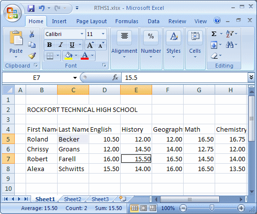
If you insert the rows, a new row would be inserted above
each selected row:
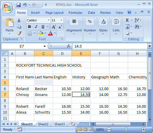
Any of these techniques adds a complete row to the list.
Sometimes, you will only want to add a new cell. You can ask Microsoft Excel to
push some cell to the right and create room for one or more new cells.
To insert a cell horizontally between two cells:
- Right-click the cell that will be pushed to the right along with the cells
on its right, and click Insert...
- Click the cell that will be pushed to the right along with its right
neighbors. On the ribbon, click Home. In the Cells section, click the arrow
button under Insert, and click Insert Cells...
Any of these actions would call the Insert dialog box. From
it, to insert a cell and push the others to the right, click the Shift Cells
Right radio button.
To undo any of these actions:
- On the Quick Access toolbar, click the Undo button

- Press Ctrl + Z
Besides adding cells, a list maintenance also consists of
deleting or moving cells. In Lesson 2, we saw how to delete one or more columns.
The problem is that, when you delete a column, all of its cells a lost. In the
same way, if you delete a row, all of its cells are lost also. Sometimes you
want to remove only one or more cells but keep the other cells of the same
column or the same row. Fortunately, Microsoft Excel supports various techniques
of removing cells from a list.
Instead of deleting a whole column, you can delete just one
cell or more cells. Because a cell is surrounded by other cells, you must
indicate what would happen to the other cells or how they would adjust to he new
empty spot.
Before deleting a cell, you first make it active. Then you
specify if, by removing it, the cells on on its right would be moved to the left
to close the left empty space. The alternative it to draw the cells from under
it up. When the cell has been removed, and the cells from the right side have
been move left, Microsoft Excel adds a new cell from the last column. If the
cells have moved up, Microsoft Excel creates a cell in the last position of that
column.
To delete a cell:
- Right-click the cell and click Delete...
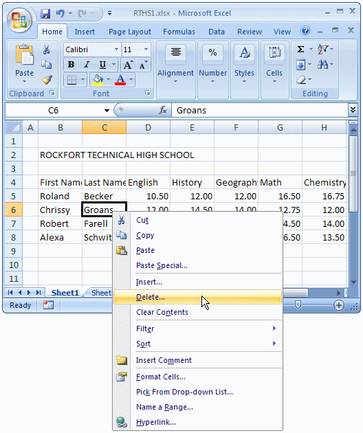
- Click the cell. On the Ribbon, click Home. In the Cells section, click
Delete and click Delete Cells...
This would display the Delete dialog box. To
To delete more than one row, first select the rows, whether
in a range or randomly. Then:
- Right-click one of the rows (whether one of the row headers or a box on the
right side of one of the selected rows) and click Delete
- (After selecting the rows,) On the Ribbon, click Home. In the Cells
section, click Delete and click Delete Sheet Rows
To undo any of these actions:
- On the Quick Access toolbar, click the Undo button

- Press Ctrl + Z
|
|

