Home

Introduction to Built-In Functions


Constants, Expressions and Formulas


Introduction to Constants

A constant is a value that does not change. It can be a number, a string, or an expression. To create a constant, use the Const keyword and assign the desired value to it. Here is an example:

Private Sub CreateConstant()
    Const Number6 = 6
End Sub

After creating the constant, you can use its name wherever its value would have been used. Some of the constants you will use in your expressions have already been created. We will mention them when necessary.

Introduction to Expressions

An expression is one or more symbols combined with one or more values to create another value. For example, +16 is an expression that creates the positive value 16. Most expressions that we know are made of arithmetic calculations. An example is 422.82 * 15.55.

To add an expression to a selected cell, assign it to the ActiveCell object. Here is an example:

Sub Exercise()
    ActiveCell = 422.82 * 15.5
End Sub

Practical LearningPractical Learning: Introducing Expressions

  1. Start Microsoft Excel
  2. On the Ribbon, click Developer
  3. In the Code section, click Record Macro
  4. Set the Macro Name to CreateWorkbook
  5. In the Shortcut Key text box, type W to get Ctrl + Shift + W and click OK
  6. On the Ribbon, click Stop Recording
  7. In the Code section of the Ribbon, click Macros Macros
  8. In the Macro dialog box, make sure CreateWorkbook is selected and click Edit
  9. Change the code as follows:
     
    Sub CreateWorkbook()
    '
    ' CreateWorkbook Macro
    ' This macro is used to create a workbook for the
    ' Georgetown Dry Cleaning Services
    '
    ' Keyboard Shortcut: Ctrl+Shift+W
    '
        Rem Just in case there is anything on the
        Rem worksheet, delete everything
        Range("A:K").Delete
        Range("1:20").Delete
        
        Rem Create the sections and headings of the worksheet
        Range("B2") = "Georgetown Dry Cleaning Services"
        Range("B2").Font.Name = "Rockwell Condensed"
        Range("B2").Font.Size = 24
        Range("B2").Font.Bold = True
        Range("B2").Font.Color = vbBlue
        
        Range("B3:J3").Interior.ThemeColor = xlThemeColorLight2
        
        Range("B5") = "Order Identification"
        Range("B5").Font.Name = "Cambria"
        Range("B5").Font.Size = 14
        Range("B5").Font.Bold = True
        Range("B5").Font.ThemeColor = 5
        
        Rem To draw a thick line, change the bottom
        Rem borders of the cells from B5 to J5
        Range("B5:J5").Borders(xlEdgeBottom).LineStyle = xlContinuous
        Range("B5:J5").Borders(xlEdgeBottom).Weight = xlMedium
        Range("B5:J5").Borders(xlEdgeBottom).ThemeColor = 5
        
        Range("B6") = "Receipt #:"
        Range("D6:F6").Borders(xlEdgeBottom).LineStyle = xlContinuous
        Range("D6:F6").Borders(xlEdgeBottom).Weight = xlHairline
        
        Range("G6") = "Order Status:"
        Range("I6:J6").Borders(xlEdgeBottom).LineStyle = xlContinuous
        Range("I6:J6").Borders(xlEdgeBottom).Weight = xlHairline
        
        Range("B7") = "Customer Name:"
        Range("D7:F7").Borders(xlEdgeBottom).LineStyle = xlContinuous
        Range("D7:F7").Borders(xlEdgeBottom).Weight = xlHairline
        
        Range("G7") = "Customer Phone:"
        Range("I7:J7").Borders(xlEdgeBottom).LineStyle = xlContinuous
        Range("I7:J7").Borders(xlEdgeBottom).Weight = xlHairline
        
        Rem To draw a thick line, change the bottom
        Rem borders of the cells from B5 to J5
        Range("B8:J8").Borders(xlEdgeBottom).LineStyle = xlContinuous
        Range("B8:J8").Borders(xlEdgeBottom).Weight = xlThin
        
        Range("B9") = "Date Left:"
        Range("D9:F9").Borders(xlEdgeBottom).LineStyle = xlContinuous
        Range("D9:F9").Borders(xlEdgeBottom).Weight = xlHairline
        
        Range("G9") = "Time Left:"
        Range("I9:J9").Borders(xlEdgeBottom).LineStyle = xlContinuous
        Range("I9:J9").Borders(xlEdgeBottom).Weight = xlHairline
        
        Range("B10") = "Date Expected:"
        Range("D10:F10").Borders(xlEdgeBottom).LineStyle = xlContinuous
        Range("D10:F10").Borders(xlEdgeBottom).Weight = xlHairline
        
        Range("G10") = "Time Expected:"
        Range("I10:J10").Borders(xlEdgeBottom).LineStyle = xlContinuous
        Range("I10:J10").Borders(xlEdgeBottom).Weight = xlHairline
        
        Range("B11") = "Date Picked Up:"
        Range("D11:F11").Borders(xlEdgeBottom).LineStyle = xlContinuous
        Range("D11:F11").Borders(xlEdgeBottom).Weight = xlHairline
        
        Range("G11") = "Time Picked Up:"
        Range("I11:J11").Borders(xlEdgeBottom).LineStyle = xlContinuous
        Range("I11:J11").Borders(xlEdgeBottom).Weight = xlHairline
        
        Rem To draw a thick line, change the bottom
        Rem borders of the cells from B5 to J5
        Range("B12:J12").Borders(xlEdgeBottom).LineStyle = xlContinuous
        Range("B12:J12").Borders(xlEdgeBottom).Weight = xlMedium
        Range("B12:J12").Borders(xlEdgeBottom).ThemeColor = 5
              
        Range("B13") = "Items to Clean"
        Range("B13").Font.Name = "Cambria"
        Range("B13").Font.Size = 14
        Range("B13").Font.Bold = True
        Range("B13").Font.ThemeColor = 5
        
        Range("B14") = "Item"
        Range("D14") = "Unit Price"
        Range("E14") = "Qty"
        Range("F14") = "Sub-Total"
        
        Range("B14:F14").Borders(xlEdgeLeft).LineStyle = xlContinuous
        Range("B14:F14").Borders(xlEdgeLeft).Weight = xlThin
        Range("B14:F14").Borders(xlEdgeTop).LineStyle = xlContinuous
        Range("B14:F14").Borders(xlEdgeTop).Weight = xlThin
        Range("B14:F14").Borders(xlEdgeRight).LineStyle = xlContinuous
        Range("B14:F14").Borders(xlEdgeRight).Weight = xlThin
        Range("B14:F14").Borders(xlEdgeBottom).LineStyle = xlContinuous
        Range("B14:F14").Borders(xlEdgeBottom).Weight = xlThin
        Range("C14").Borders(xlEdgeRight).LineStyle = xlContinuous
        Range("C14").Borders(xlEdgeRight).Weight = xlThin
        Range("D14").Borders(xlEdgeRight).LineStyle = xlContinuous
        Range("D14").Borders(xlEdgeRight).Weight = xlThin
        Range("E14").Borders(xlEdgeRight).LineStyle = xlContinuous
        Range("E14").Borders(xlEdgeRight).Weight = xlThin
    
        Range("B15") = "Shirts"
        Range("B15").Borders(xlEdgeLeft).LineStyle = xlContinuous
        Range("B15").Borders(xlEdgeLeft).Weight = xlThin
        
        Range("H15") = "Order Summary"
        Range("H15").Font.Name = "Cambria"
        Range("H15").Font.Size = 14
        Range("H15").Font.Bold = True
        Range("H15").Font.ThemeColor = 5
        
        Range("B16") = "Pants"
        Range("B16").Borders(xlEdgeLeft).LineStyle = xlContinuous
        Range("B16").Borders(xlEdgeLeft).Weight = xlThin
        
        Range("B17") = "None"
        Range("B17").Borders(xlEdgeLeft).LineStyle = xlContinuous
        Range("B17").Borders(xlEdgeLeft).Weight = xlThin
        
        Range("H17") = "Cleaning Total:"
        Range("I17").Borders(xlEdgeBottom).LineStyle = xlContinuous
        Range("I17").Borders(xlEdgeBottom).Weight = xlHairline
        
        Range("B18") = "None"
        Range("B18").Borders(xlEdgeLeft).LineStyle = xlContinuous
        Range("B18").Borders(xlEdgeLeft).Weight = xlThin
        
        Range("H18") = "Tax Rate:"
        Range("I18").Borders(xlEdgeBottom).LineStyle = xlContinuous
        Range("I18").Borders(xlEdgeBottom).Weight = xlHairline
        
        Range("I18") = "5.75"
        Range("J18") = "%"
        Range("B19") = "None"
        Range("B19").Borders(xlEdgeLeft).LineStyle = xlContinuous
        Range("B19").Borders(xlEdgeLeft).Weight = xlThin
        
        Range("H19") = "Tax Amount:"
        Range("I19").Borders(xlEdgeBottom).LineStyle = xlContinuous
        Range("I19").Borders(xlEdgeBottom).Weight = xlHairline
        
        Range("B20") = "None"
        Range("B20").Borders(xlEdgeLeft).LineStyle = xlContinuous
        Range("B20").Borders(xlEdgeLeft).Weight = xlThin
        
        Range("C15").Borders(xlEdgeRight).LineStyle = xlContinuous
        Range("C15").Borders(xlEdgeRight).Weight = xlThin
        Range("C16").Borders(xlEdgeRight).LineStyle = xlContinuous
        Range("C16").Borders(xlEdgeRight).Weight = xlThin
        Range("C17").Borders(xlEdgeRight).LineStyle = xlContinuous
        Range("C17").Borders(xlEdgeRight).Weight = xlThin
        Range("C18").Borders(xlEdgeRight).LineStyle = xlContinuous
        Range("C18").Borders(xlEdgeRight).Weight = xlThin
        Range("C19").Borders(xlEdgeRight).LineStyle = xlContinuous
        Range("C19").Borders(xlEdgeRight).Weight = xlThin
        Range("C20").Borders(xlEdgeRight).LineStyle = xlContinuous
        Range("C20").Borders(xlEdgeRight).Weight = xlThin
        Range("B14:C14").Borders(xlEdgeBottom).LineStyle = xlContinuous
        Range("B14:C14").Borders(xlEdgeBottom).Weight = xlThin
        
        Range("B15:C15").Borders(xlEdgeBottom).LineStyle = xlContinuous
        Range("B15:C15").Borders(xlEdgeBottom).Weight = xlThin
        Range("D15:F15").Borders(xlEdgeBottom).LineStyle = xlContinuous
        Range("D15:F15").Borders(xlEdgeBottom).Weight = xlHairline
        Range("D15").Borders(xlEdgeRight).LineStyle = xlContinuous
        Range("D15").Borders(xlEdgeRight).Weight = xlHairline
        Range("E15").Borders(xlEdgeRight).LineStyle = xlContinuous
        Range("E15").Borders(xlEdgeRight).Weight = xlHairline
        Range("F15").Borders(xlEdgeRight).LineStyle = xlContinuous
        Range("F15").Borders(xlEdgeRight).Weight = xlThin
        
        Range("B16:C16").Borders(xlEdgeBottom).LineStyle = xlContinuous
        Range("B16:C16").Borders(xlEdgeBottom).Weight = xlThin
        Range("D16:F16").Borders(xlEdgeBottom).LineStyle = xlContinuous
        Range("D16:F16").Borders(xlEdgeBottom).Weight = xlHairline
        Range("D16").Borders(xlEdgeRight).LineStyle = xlContinuous
        Range("D16").Borders(xlEdgeRight).Weight = xlHairline
        Range("E16").Borders(xlEdgeRight).LineStyle = xlContinuous
        Range("E16").Borders(xlEdgeRight).Weight = xlHairline
        Range("F16").Borders(xlEdgeRight).LineStyle = xlContinuous
        Range("F16").Borders(xlEdgeRight).Weight = xlThin
        
        Range("B17:C17").Borders(xlEdgeBottom).LineStyle = xlContinuous
        Range("B17:C17").Borders(xlEdgeBottom).Weight = xlThin
        Range("D17:F17").Borders(xlEdgeBottom).LineStyle = xlContinuous
        Range("D17:F17").Borders(xlEdgeBottom).Weight = xlHairline
        Range("D17").Borders(xlEdgeRight).LineStyle = xlContinuous
        Range("D17").Borders(xlEdgeRight).Weight = xlHairline
        Range("E17").Borders(xlEdgeRight).LineStyle = xlContinuous
        Range("E17").Borders(xlEdgeRight).Weight = xlHairline
        Range("F17").Borders(xlEdgeRight).LineStyle = xlContinuous
        Range("F17").Borders(xlEdgeRight).Weight = xlThin
        
        Range("B18:C18").Borders(xlEdgeBottom).LineStyle = xlContinuous
        Range("B18:C18").Borders(xlEdgeBottom).Weight = xlThin
        Range("D18:F18").Borders(xlEdgeBottom).LineStyle = xlContinuous
        Range("D18:F18").Borders(xlEdgeBottom).Weight = xlHairline
        Range("D18").Borders(xlEdgeRight).LineStyle = xlContinuous
        Range("D18").Borders(xlEdgeRight).Weight = xlHairline
        Range("E18").Borders(xlEdgeRight).LineStyle = xlContinuous
        Range("E18").Borders(xlEdgeRight).Weight = xlHairline
        Range("F18").Borders(xlEdgeRight).LineStyle = xlContinuous
        Range("F18").Borders(xlEdgeRight).Weight = xlThin
        
        Range("B19:C19").Borders(xlEdgeBottom).LineStyle = xlContinuous
        Range("B19:C19").Borders(xlEdgeBottom).Weight = xlThin
        Range("D19:F19").Borders(xlEdgeBottom).LineStyle = xlContinuous
        Range("D19:F19").Borders(xlEdgeBottom).Weight = xlHairline
        Range("D19").Borders(xlEdgeRight).LineStyle = xlContinuous
        Range("D19").Borders(xlEdgeRight).Weight = xlHairline
        Range("E19").Borders(xlEdgeRight).LineStyle = xlContinuous
        Range("E19").Borders(xlEdgeRight).Weight = xlHairline
        Range("F19").Borders(xlEdgeRight).LineStyle = xlContinuous
        Range("F19").Borders(xlEdgeRight).Weight = xlThin
        
        Range("B20:F20").Borders(xlEdgeBottom).LineStyle = xlContinuous
        Range("B20:F20").Borders(xlEdgeBottom).Weight = xlThin
        Range("D20").Borders(xlEdgeRight).LineStyle = xlContinuous
        Range("D20").Borders(xlEdgeRight).Weight = xlHairline
        Range("E20").Borders(xlEdgeRight).LineStyle = xlContinuous
        Range("E20").Borders(xlEdgeRight).Weight = xlHairline
        Range("F20").Borders(xlEdgeRight).LineStyle = xlContinuous
        Range("F20").Borders(xlEdgeRight).Weight = xlThin
        
        Range("H20") = "Order Total:"
        Range("I20").Borders(xlEdgeBottom).LineStyle = xlContinuous
        Range("I20").Borders(xlEdgeBottom).Weight = xlHairline
        
        Rem Change the widths and heights of some columns and rows
        Rem In previous lessons, we learned all these things
        Range("E:E, G:G").ColumnWidth = 4
        Columns("H").ColumnWidth = 14
        Columns("J").ColumnWidth = 1.75
        
        Rows("3").RowHeight = 2
        Range("8:8, 12:12").RowHeight = 8
        
        Rem Merge the cells H15, I15, H16, and I16
        Range("H15:I16").MergeCells = True
        Rem Align the merged text to the left
        Range("H15:H16").VerticalAlignment = xlBottom
        
        Range("H16").Borders(xlEdgeBottom).LineStyle = xlContinuous
        Range("H16:I16").Borders(xlEdgeBottom).Weight = xlMedium
        Range("H16:I16").Borders(xlEdgeBottom).ThemeColor = 5
        
        Rem Hide the gridlines
        ActiveWindow.DisplayGridlines = False
    End Sub
  10. To return to Microsoft Excel, click the View Microsoft Excel button View Microsoft Excel
  11. To fill the worksheet, press Ctrl + Shift + W

Introduction to Formulas

A formula is another name for an expression. It combines one or more values, one or more variables, to an operator, to produce a new value. This also means that you use the same approach or building an expression when creating a formula.

To assist you with assigning the result of a formula to a cell or a group of cells, the Range class is equipped with a property named Formula. This property is of type Variant, which means its value can be anything, not necessarily a number. After accessing the Formula property, you can assign whatever value, expression, or formula you want to it. Here are examples:

Sub Exercise()
    Rem Using the Formula property to assign a string to the active cell
    ActiveCell.Formula = "Weekly Salary:"
    
    Rem Using the Formula property to assign an expression to cell B2
    Range("B2").Formula = 24.5 * 42.5
    
    Rem  Using the Formula property to assign
    Rem the same string to a group of cells
    Range("C2:F5, B8:D12").Formula = "Antoinette"
End Sub

If you are creating a worksheet that would be used on computers of different languages, use FormulaLocal instead. The FormulaLocal property is equipped to adapt to a different language-based version of Microsoft Excel when necessary.

Besides Formula, the Range class is also equipped with a property named FormulaR1C1. Its functionality is primarily the same as Formula. Here are examples:

Sub Exercise()
    Rem Using the Formula property to assign a string to the active cell
    ActiveCell.FormulaR1C1 = "Weekly Salary:"
    
    Rem Using the Formula property to assign an expression to cell B2
    Range("B2").FormulaR1C1 = 24.5 * 42.5
    
    Rem  Using the Formula property to assign
    Rem the same string to a group of cells
    Range("C2:F5, B8:D12").FormulaR1C1 = "Antoinette"
End Sub

If you are creating the worksheet for various languages, use FormulaR1C1Local instead.

Practical Learning: Creating Formulas

  1. In the Developer tab of the Ribbon and in the Code section, click Record Macro
  2. Set the Macro Name to CalculateOrder
  3. In the Shortcut Key text box, type C to get Ctrl + Shift + C
     
  4. Click OK
  5. On the Ribbon, click Stop Recording
  6. In the Code section of the Ribbon, click Macros Macros
  7. In the Macro dialog box, make sure CalculateOrder is selected and click Edit
  8. Change the code as follows:
     
    Sub CalculateOrder()
    '
    ' CreateWorkbook Macro
    '
    ' Keyboard Shortcut: Ctrl+Shift+C
    '
        Rem Calculate the sub-total of each category of items as:
        Rem SubTotal = Unit Price * Quantity
        Rem And display the total in the equivalent F cell
        Range("F15").Formula = Range("D15") * Range("E15")
        Range("F16").Formula = Range("D16") * Range("E16")
        Range("F17").Formula = Range("D17") * Range("E17")
        Range("F18").Formula = Range("D18") * Range("E18")
        Range("F19").Formula = Range("D19") * Range("E19")
        Range("F20").Formula = Range("D20") * Range("E20")
        
        Rem Retrieve the values of the cleaning total and the tax rate
        Rem Use them to calculate the amount of tax
        Range("I19").Formula = Range("I17") * Range("I18") / 100
        
        Rem Calculate the total order by adding 
        Rem the cleaning total to the tax amount
        Range("I20").Formula = Range("I17") + Range("I19")
    End Sub

Fundamentals of Built-In Functions


Introduction

Instead of creating your own function, you can use one of those that ship with the VBA language. This language provides a very extensive library of functions so that, before creating your own, check whether the function exists already. If so, use it instead.

To use a VBA built-in function, simply use as you would an expression. That is, assign its returned value to a cell. Here is an example:

Sub Exercise()
    Range("B2:B2") = Len("Paul Bertrand Yamaguchi")
End Sub

Microsoft Excel Built-In Functions

To assist you with developing smart worksheets, Microsoft Excel provides a very large library of functions. To use a Microsoft Excel built-in function in your code, you have many functions.

In double-quotes, you can include the assignment operator followed by the function's whole expression. Here is an example:

Sub Exercise()
    Range("B5:B5") = "=SomeFunction(B2, B3, B4)"
End Sub

As an alternative, the Application class is equipped with a property named WorksheetFunction. This property represents all functions of the Microsoft Excel library. Therefore, to access a function, type Application, followed by a period, followed by a period. Then type (or select the name of the function you want to use:
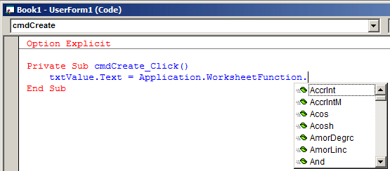
Code Editor

After specifying the function you want to use, because it is a function, you must include the parentheses. In the parentheses, type the necessary argument(s). Here is an example:

Private Sub cmdCreate_Click()
    txtValue.Text = Application.WorksheetFunction.Sum(Range("D4:D8"))
End Sub

Conversion Functions

You may recall that when studying data types, we saw that each had a corresponding function used to convert a string value or an expression to that type. As a reminder, the general syntax of the conversion functions is:

ReturnType = FunctionName(Expression)

The Expression could be of any kind. For example, it could be a string or expression that would produce a value such as the result of a calculation. The conversion function would take such a value, string, or expression and attempt to convert it. If the conversion is successful, the function would return a new value that is of the type specified by the ReturnType in our syntax.

The conversion functions are as follows:

Function  
Name Return Type Description
CBool Boolean Converts an expression into a Boolean value
CByte Byte Converts an expression into Byte number
CDbl Double Converts an expression into a floating-point number with double precision
CDec Decimal Converts an expression into a decimal number
CInt Integer Converts an expression into an integer (natural) number
CLng Long Converts an expression into a long integer (a large natural) number
CObj Object Converts an expression into an Object type
CSByte SByte Converts an expression into a signed byte
CShort Short Converts an expression into a short integer
CSng Single Converts an expression into a floating-point number with single precision
CUInt UInt Converts an expression into an unsigned integer
CULng ULong Converts an expression into an unsigned long integer
CUShort UShort Converts an expression into an unsigned short integer

These functions allow you to convert a known value to a another type.

Practical Learning: Using Conversion Functions

  • Change the code as follows:
     
    Sub CalculateOrder()
    '
    ' CalculateOrder Macro
    '
    ' Keyboard Shortcut: Ctrl+Shift+C
        
        Rem Calculate the sub-total of each category of items as:
        Rem SubTotal = Unit Price * Quantity
        Rem And display the total in the equivalent F cell
        Range("F15").Formula = CDbl(Range("D15")) * CInt(Range("E15"))
        Range("F16").Formula = CDbl(Range("D16")) * CInt(Range("E16"))
        Range("F17").Formula = CDbl(Range("D17")) * CInt(Range("E17"))
        Range("F18").Formula = CDbl(Range("D18")) * CInt(Range("E18"))
        Range("F19").Formula = CDbl(Range("D19")) * CInt(Range("E19"))
        Range("F20").Formula = CDbl(Range("D20")) * CInt(Range("E20"))
        
        Rem Retrieve the values of the cleaning total and the tax rate
        Rem Use them to calculate the amount of tax
        Range("I19").Formula = CDbl(Range("I17")) * CDbl(Range("I18")) / 100
        
        Rem Calculate the total order by adding the
        Rem cleaning total to the tax amount
        Range("I20").Formula = CDbl(Range("I17")) + CDbl(Range("I19"))
    End Sub


Accessory Built-In Functions


Introduction

Both Microsoft Excel and the Visual Basic language provide each an extensive library of functions. We refer to some functions as accessories because you almost cannot anything about them or at least they are very useful.

Specifying a Color

To assist you with specifying the color of anything, the VBA is equipped with a function named RGB. Its syntax is:

Function RGB(RedValue As Byte, GreenValue As Byte, BlueValue As Byte) As long

This function takes three arguments and each must hold a value between 0 and 255. The first argument represents the ratio of red of the color. The second argument represents the green ratio of the color. The last argument represents the blue of the color. After the function has been called, it produces a number whose maximum value can be 255 * 255 * 255 = 16,581,375, which represents a color.

Practical Learning: Using the RGB Function

  1. Locate the CreateWorkbook procedure and change its code as follows:
     
    Sub CreateWorkbook()
    '
    ' CreateWorkbook Macro
    '
    ' Keyboard Shortcut: Ctrl+Shift+E
    '
        . . . No Change
        
        Rem Change the background color of cells F15 to F20 to a light blue
        Range("F15:F20").Interior.Color = RGB(210, 225, 250)
        Rem Change the background color of cells I17 to I20 to a dark blue
        Range("I17:I20").Interior.Color = RGB(5, 65, 165)
        Rem Change the text color of cells I17 to I20 to a dark blue
        Range("I17:I20").Font.Color = RGB(255, 255, 195)
        
        Rem Hide the gridlines
        ActiveWindow.DisplayGridlines = False
    End Sub
  2. Return to Microsoft Excel and press Ctrl + Shift + W
  3. Press Ctrl + Shift + C to see the result
     
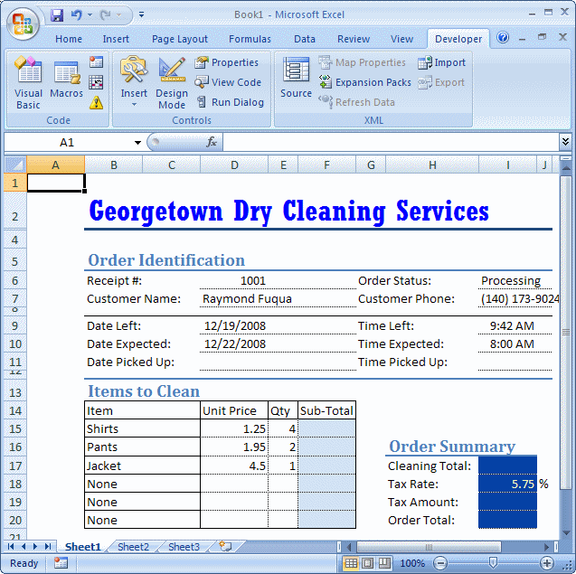
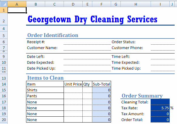
    Georgetown Dry Cleaning Services
  4. Return to Microsoft Visual Basic

The Sum Function

The Microsoft Excel's SUM function is used to add the numeric values of various cells. The result can be displayed in another cell or used in an expression. Like all functions of the Microsoft Excel library, you can use SUM visually or programmatically.

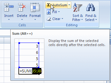
To use the SUM() function visually, on the Ribbon, in the Home tab, the Editing section is equipped with a button called the AutoSum

AutoSum

Practical Learning: Using the SUM Function

  1. Locate the CalculateOrder procedure and change its code as follows:
     
    Sub CalculateOrder()
    '
    ' CalculateOrder Macro
    '
    ' Keyboard Shortcut: Ctrl+Shift+C
    '
        Rem Calculate the sub-total of each category of items as:
        Rem SubTotal = Unit Price * Quantity
        Rem And display the total in the equivalent F cell
        Range("F15").Formula = CDbl(Range("D15")) * CInt(Range("E15"))
        Range("F16").Formula = CDbl(Range("D16")) * CInt(Range("E16"))
        Range("F17").Formula = CDbl(Range("D17")) * CInt(Range("E17"))
        Range("F18").Formula = CDbl(Range("D18")) * CInt(Range("E18"))
        Range("F19").Formula = CDbl(Range("D19")) * CInt(Range("E19"))
        Range("F20").Formula = CDbl(Range("D20")) * CInt(Range("E20"))
        
        Rem Use the SUM() function to calculate the sum of
        Rem cells F15 to F20 and display the result in cell J17
        Range("I17").Formula = "=SUM(F15:F20)"
        
        Rem Retrieve the values of the cleaning total and the tax rate
        Rem Use them to calculate the amount of tax
        Range("I19").Formula = CDbl(Range("I17")) * CDbl(Range("I18")) / 100
        
        Rem Calculate the total order by adding the
        Rem cleaning total to the tax amount
        Range("I20").Formula = CDbl(Range("I17")) + CDbl(Range("I19"))
    End Sub
  2. Return to Microsoft Excel and press Ctrl + Shift + C to see the result
  3. Enter the following values in the worksheet:
     
    Receipt #: 1001 Order Status: Processing
    Customer Name: Raymond Fuqua Customer Phone: (140) 173-9024
    Date Left: 12/19/2008 Time Left: 09:42 AM
    Date Expected: 12/22/2008 Time Expected: 08:00 AM
     
      Unit Price Qty
    Shirts 1.25 4
    Pants 1.95 2
    Jacket 4.50 1
  4. Click cell A1
     
    Georgetown Dry Cleaning Services
  5. Press Ctrl + Shift + C
     
    Georgetown Dry Cleaning Services
  6. Return to Microsoft Visual Basic

The Absolute Value

The absolute value of a number x is x if the number is (already) positive. If the number is negative, then its absolute value is its positive equivalent. For example, the absolute value of 12 is 12, while the absolute value of –12 is 12.

To get the absolute value of a number, you can use either the Microsoft Excel's ABS() or the VBA's Abs() function. Their syntaxes are:

Function ABS(number) As Number
Function Abs(number) As Number

This function takes one argument. The argument must be a number or an expression convertible to a number:

  • If the argument is a positive number, the function returns it
  • If the argument is zero, the function returns 0
  • If the argument is a negative number, the function is returns its equivalent positive value

Getting the Integral Part of a Number

If you have a decimal number but are interested only in the integral part, to assist you with retrieving that part, the Visual Basic language provides the Int() and the Fix() functions. In the same way, the Microsoft Excel library provides the INT() function to perform a similar operation. Their syntaxes are:

Function Int(ByVal Number As { Number | Expression } ) As Integer
Function Fix(ByVal Number As { Number | Expression } ) As Integer
Function ABS(ByVal Number As { Number | Expression } ) As Integer

Each function must take one argument. The value of the argument must be number-based. This means it can be an integer or a floating-point number. If the value of the argument is integer-based, the function returns the (whole) number. Here is an example

Sub Exercise()
    Dim Number As Integer

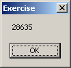
    Number = 28635
    ActiveCell = MsgBox(Int(Number), vbOKOnly, "Exercise")
End Sub

This would produce:

Int

If the value of the argument is a decimal number, the function returns only the integral part. Here is an example

Sub Exercise()
    Dim Number As Double

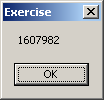
    Number = 7942.225 * 202.46
    ActiveCell = MsgBox(Int(Number), vbOKOnly, "Exercise")
End Sub

This would produce:

Int

This function always returns the integral part only, even if you ask it to return a floating-point-based value. Here is an example:

Sub Exercise()
    Dim Number As Single

    Number = 286345.9924
    ActiveCell = MsgBox(Int(Number), vbOKOnly, "Exercise")
End Sub

This would produce:

Int

Cells Content Formatting


Introduction

When it receive values for its cells, by default, Microsoft Excel displays text left aligned and numbers right aligned. In some situations, you will want to treat numbers as text.

Although Microsoft Excel displays all numbers right aligned, as a smart financial and business application, it can distinguish between different types of numbers. It can recognize a date, a currency, or a percentage values, but the computer wants you to specify the way numbers should be displayed, giving you the ability to decide what a particular number represents, not because the software cannot recognize a number, but because a value can represent different things to different people in different scenarios. For example 1.5 might represent a half teaspoon in one spreadsheet while the same 1.5 would represent somebody's age, another spreadsheet's percentage, or etc.

Introduction to Numbers Formatting

When it comes to displaying items, Microsoft Excel uses various default configurations. The computer's Regional Options or Regional Settings govern how dates, numbers, and time, etc get displayed on your computer.

Microsoft Excel recognizes numbers in various formats: accounting, scientific, fractions, and currency. As the software product can recognize a number, you still have the ability to display the number with a format that suits a particular scenario.

To visually control how a cell should display its number, on the Ribbon, click Home and use the Number section.

To assist you with programmatically specifying how a cell should display its number, the Range class is equipped with a property named Style.

To further assist with number formatting, the Visual Basic language provides a function named Format. This function can be used for different types of values The most basic technique consists of passing it an expression that holds the value to display. The syntax of this function is:

Function Format(ByVal Expression As Variant, _
   Optional ByVal Style As String = "" _
) As String

The first argument is the value that must be formatted. Here is an example:

Sub Exercise()
    Dim Number As Double

    Number = 20502.48
    ActiveCell = Format(Number)
End Sub

The second argument is optionally. It specifies the type of format you want to apply. We will see various examples.

Formatting a Number

To visually specify that you want a cell to display its numeric value with the comma delimiter, click the cell to give it focus. Then, in the Home tab of the Ribbon, in the Number section, click the Comma Style button Comma Style. The thousand numbers would display with a comma sign which makes it easier to read.

To visually control the number of decimal values on the right side of the comma, in the Number section of the Ribbon:

  • You can click the Decrease Decimal button to remove one decimal value. You can continuously click the Decrease Decimal button to decrease the number of digits.
  • You can click the Increase Decimal button Increase Decimal  to increase the number of digits

To programmatically specify that you want a cell to display the comma style of number, assign the "Comma" string to the Style property of the Range class. Here is an example:

Sub SpecifyComma()
    ActiveCell.Style = "Comma"
End Sub

Alternatively, to programmatically control how the number should display, you can pass the second argument to the Format() function. To produce the number in a general format, you can pass the second argument as "g", "G", "f", or "F" .

To display the number with a decimal separator, pass the second argument as "n", "N", or "Standard". Here is an example:

Sub Exercise()
    Dim Number As Double

    Number = 20502.48
    ActiveCell = Format(Number, "STANDARD")
End Sub

An alternative to get this format is to call a function named FormatNumber. Its syntax is:

Function FormatNumber(
   ByVal Expression As Variant,
   Optional ByVal NumDigitsAfterDecimal As Integer = -1,
   Optional ByVal IncludeLeadingDigit As Integer,
   Optional ByVal UseParensForNegativeNumbers As Integer,
   Optional ByVal GroupDigits As Integer
) As String

Only the first argument is required and it represents the value to display. If you pass only this argument, you get the same format as the Format() function called with the Standard option. Here is an example:

Sub Exercise()
    Dim Number As Double

    Number = 20502.48
    ActiveCell = FormatNumber(Number)
End Sub

This would produce the same result as above.

If you call the Format() function with the Standard option, it would consider only the number of digits on the right side of the decimal separator. If you want to display more digits than the number actually has, call the FormatNumber() function and pass a second argument with the desired number. Here is an example:

Sub Exercise()
    Dim Number As Double

    Number = 20502.48
    ActiveCell = FormatNumber(Number, 4)
End Sub

In the same way, if you want the number to display with less numbers on the right side of the decimal separator, specify that number.

We saw that you could click the Decrease Decimal button on the Ribbon to visually control the number of decimal values on the right side of the comma and you could continuously click that button to decrease the number of digits. Of course, you can also exercise this control programmatically.

You can call the Format() function to format the number with many more options. To represent the integral part of a number, you use the # sign. To specify the number of digits to display on the right side of the decimal separator, type a period on the right side of # followed by the number of 0s representing each decimal place. Here is an example:

Sub Exercise()
    Dim Number As Double

    Number = 20502.48
    ActiveCell = Format(Number, "#.00000")
End Sub

The five 0s on the right side of the period indicate that you want to display 5 digits on the right side of the period. You can enter as many # signs as you want; it would not change anything. Here is an example:

Sub Exercise()
    Dim Number As Double

    Number = 20502.48
    ActiveCell = Format(Number, "##########.00000")
End Sub

This would produce the same result as above. To specify that you want to display the decimal separator, include its character between the # signs. Here is an example:

Sub Exercise()
    Dim Number As Double

    Number = 20502.48
    ActiveCell = Format(Number, "###,#######.00000")
End Sub

You can include any other character or symbol you want in the string to be part of the result, but you should include such a character only at the beginning or the end of the string, otherwise the interpreter might give you an unexpected result.

Practical Learning: Using the SUM Function

  1. Locate the CreateWorkbook procedure and change its code as follows:
     
    Sub CreateWorkbook()
    '
    ' CreateWorkbook Macro
    '
    ' Keyboard Shortcut: Ctrl+Shift+W
    '
        . . . No Change
        
        Rem Format the values in the unit prices
        Range("D15").Style = "Comma"
        Range("D16").Style = "Comma"
        Range("D17").Style = "Comma"
        Range("D18").Style = "Comma"
        Range("D19").Style = "Comma"
        Range("D20").Style = "Comma"
        
        Rem Format the values in the sub totals
        Range("F15").Style = "Comma"
        Range("F16").Style = "Comma"
        Range("F17").Style = "Comma"
        Range("F18").Style = "Comma"
        Range("F19").Style = "Comma"
        Range("F20").Style = "Comma"
        
        Rem Format the values in the Order Summary section
        Range("I17").Style = "Comma"
        Range("I19").Style = "Comma"
        Range("I20").Style = "Comma"
        
        Rem Hide the gridlines
        ActiveWindow.DisplayGridlines = False
    End Sub
  2. Return to Microsoft Excel and press Ctrl + Shift + W
  3. Enter the following values in the worksheet:
     
    Receipt #: 1001 Order Status: Processing
    Customer Name: Raymond Fuqua Customer Phone: (140) 173-9024
    Date Left: 12/19/2008 Time Left: 09:42 AM
    Date Expected: 12/22/2008 Time Expected: 08:00 AM
     
      Unit Price Qty
    Shirts 1.25 4
    Pants 1.95 2
    Jacket 4.50 1
  4. Click cell A1
     
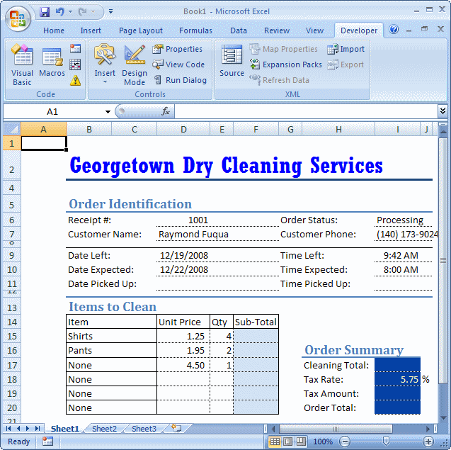
    Georgetown Dry Cleaning Services
  5. Press Ctrl + Shift + C
     
    Georgetown Dry Cleaning Services
  6. Return to Microsoft Visual Basic

Formatting a Currency Value

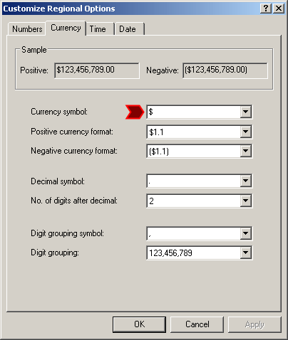
Another regular type of number used in applications and finances is the currency. A currency value uses a special character specified in the Control Panel. In US English, this character would be the $ sign:

Currency

To visually that a cell should display its number as currency, in the Number section of the Ribbon, click the Currency Style button Currency.

To programmatically specify that you want a cell to display its value with the currency style, assign the "Currency" string to the Style property of the Range class. Here is an example:

Sub SpecifyComma()
    ActiveCell.Style = "Currency"
End Sub

Alternatively, to programmatically display the currency symbol in the result of a cell or a text box of a form, you can simply add it as part of the second argument to the Format() function. Here is an example:

Sub Exercise()
    Dim Number As Double

    Number = 205.5

    ActiveCell = Format(Number, "$###,#######.00")
End Sub

Fortunately, there are more professional options. Besides the Format() function, to support currency formatting of a number, the Visual Basic language provides the FormatCurrency() function. Its syntax is:

Function FormatCurrency(
   ByVal Expression As Variant,
   Optional ByVal NumDigitsAfterDecimal As Integer = -1,
   Optional ByVal IncludeLeadingDigit As Integer = -2,
   Optional ByVal UseParensForNegativeNumbers As Integer = -2,
   Optional ByVal GroupDigits As Integer = -2
) As String

Only the first argument is required. It is the value that needs to be formatted. Here is an example:

Sub Exercise()
    Dim UnitPrice As Double

    UnitPrice = 1450.5

    ActiveCell = FormatCurrency(UnitPrice)
End Sub

Notice that, by default, the FormatCurrency() function is equipped to display the currency symbol (which, in US English is, the $ sign), the decimal separator (which in US English is the comma), and two decimal digits. If you want to control how many decimal digits are given to the result, pass a second argument as an integer. Here is an example:

Sub Exercise()
    Dim UnitPrice As Double

    UnitPrice = 1450.5

    ActiveCell = FormatCurrency(UnitPrice, 4)
End Sub

Instead of calling the FormatCurrency() function to format a number to currency, you can use the Format() function. If you do, pass it a second argument as "Currency", "c", or "C". Here is an example:

Sub Exercise()
    Dim CarPrice As Double

    CarPrice = 42790

    ActiveCell = Format(CarPrice, "Currency")
End Sub

Formatting a Percentage Value

A percentage of a number represents its rate on a scale, usually of 100 (or more). The number is expressed using digits accompanied by the % sign. To visually specify that a number in a cell should be treated a percentage value, in the Number section of the Ribbon, click the Percent Style button .

To programmatically use a percentage number in a cell or the control of a form, you can use the Format() function. Besides the Format() function, to support percent values, the Visual Basic language provides a function named FormatPercent. Its syntax is:

Function FormatPercent(
   ByVal Expression As Variant,
   Optional ByVal NumDigitsAfterDecimal As Integer = -1,
   Optional ByVal IncludeLeadingDigit As Integer = -2,
   Optional ByVal UseParensForNegativeNumbers As Integer = -2,
   Optional ByVal GroupDigits As Integer = -2
) As String

Only the first argument is required and it is the number that needs to be formatted. When calling this function, pay attention to the number you provide as argument. If the number represents a percentage value as a fraction of 0 to 1, make sure you provide it as such. An example would be 0.25. In this case, the Visual Basic interpreter would multiply the value by 100 to give the result. Here is an example:

Sub Exercise()
    Dim DiscountRate As Double

    DiscountRate = 0.25
    ActiveCell = FormatPercent(DiscountRate)
End Sub

If you pass the value in the hundreds, the interpreter would still multiply it by 100. Although it is not impossible to get a percentage value in the hundreds or thousands, you should make sure that's the type of value you mean to get.

Besides the FormatPercent() function, to format a number to its percentage equivalent, you can call the Format() function and pass the second argument as "Percent", "p", or "P". Here is an example:

Sub Exercise()
    Dim DiscountRate As Double

    DiscountRate = 0.25
    ActiveCell = MsgBox("Discount Rate: " & _
		      Format(DiscountRate, "Percent"), _
		      vbOKOnly, "Exercise")
End Sub

Number Format Options

Although you can do most of cells configurations using the Ribbon, Microsoft Excel provides the Format Cells dialog box. This dialog box presents more options and more precision.

To display the Format Cells dialog box:

  • On the Ribbon, click Home. In the Number section, click the more options button:

Number

  • Right-click the cell or group of cells whose format you want to change and click Format Cells...
  • Press Ctrl + 1 as a shortcut


Previous Copyright © 2008-2016, FunctionX, Inc. Next